Gang Bao,, Yide Zhang, Student, and Zhigang Zeng,

Abstract—Traditional recurrent neural networks are composed of capacitors, inductors, resistors, and operational amplifiers.Memristive neural networks are constructed by replacing resistors with memristors. This paper focuses on the memory analysis,i.e. the initial value computation, of memristors. Firstly, we present the memory analysis for a single memristor based on memristors' mathematical models with linear and nonlinear drift.Secondly, we present the memory analysis for two memristors in series and parallel. Thirdly, we point out the difference between traditional neural networks and those that are memristive. Based on the current and voltage relationship of memristors, we use mathematical analysis and SPICE simulations to demonstrate the validity of our methods.

I. INTRODUCTION

THE memristor was first defined by Chua [1] and can be described by the following mathematical model [2]

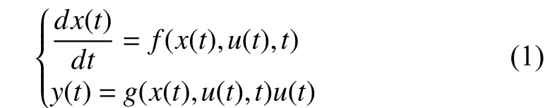
whereu(t),y(t) are input and output of memristive systems,respectively.x(t) is the state variable,f(x(t),u(t),t) is an-dimensional vector function andg(x(t),u(t),t) is the generalized system response. Williams and his colleagues transform the concept of memristors into the physical devices [3], whose structure diagram is shown in Fig. 1. The memristor is composed of a two-layer TiO2thin film, two platinum contacts, a doped regionRon, and an undoped regionRoff.D,ware the thickness of the film and the width of the doped region, respectively. Later, Chua points out that all two-terminal nonvolatile memory devices based on resistance switching are memristors, regardless of the device material and physical operating mechanisms [4].

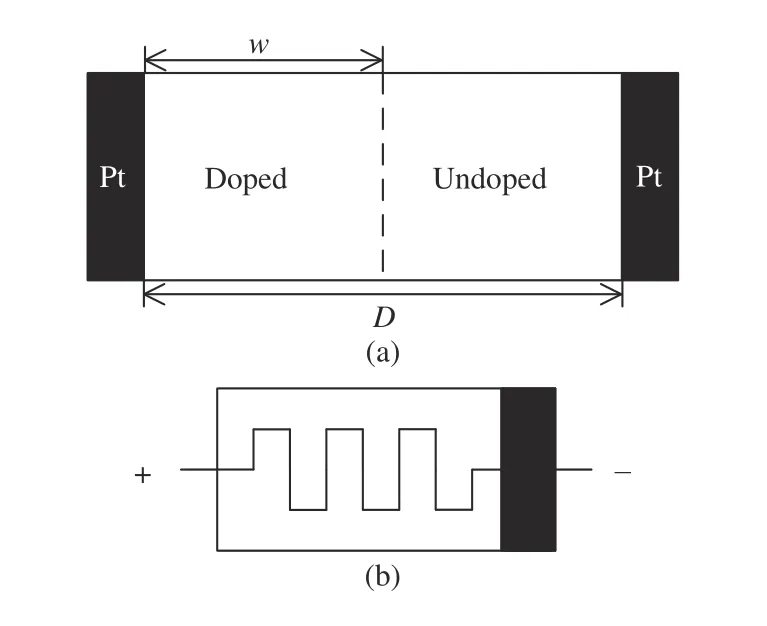
Fig. 1. The schematic diagram of the HP memristor. (a) The diagram of the HP memristor model. (b) The circuit symbol of the memristor, showing the positive and negative polarities.

The memristor has various applications for its nano-scale size and memory property. For example, it is used to implement chaotic circuits [5], [6], memristor oscillators [7],and neural synapses [8]. Snideret al. adopt memristors in neuromorphic applications to simulate learning, adaptive and spontaneous behaviors and to implement synaptic weights in artificial neural networks [9], [10]. Pershin and Di Ventra give an experimental demonstration for associative memory with memristive neural networks [11]. Then the memristor is employed as a nonvolatile memory storage device [12], [13].Furthermore, it has also been used to simulate the human brain’s hierarchical temporal memory, short-term, long-term memory [14], [15] and memristive recurrent neural networks.Meanwhile, memristors have also been harnessed for image processing, adaptive filters, digital logic, neuromophic engineering, digital and quantum computation [16], [17], etc.

The dynamic properties of memristors are the foundation for its applications; thus memristors with different materials and configurations are made for dynamic analysis experiments [18],[19]. Williamset al. [3] present the mathematical model for memristors and show its fingerprint characteristic with a pinched hysteresis currenti-voltagevloop. Based on Williams’mathematical model of memristors, Wang [20] derives the formula of the internal statex(t) and obtains the analytical expression of the currenti(t) and the voltagev(t). Considering the doped materials’ nonlinear drift, Bioleket al. [21] introduce window functions and give the SPICE model of memristors.Using Bernoulli dynamics, Drakakiset al. [22]derive the analytic description,Imres=f(Vmres) which defines the relation between the currentImresand the voltageVmresunder the assumption of nonlinear dopant drift. Wanget al. [23]and Zhanget al. [24] propose a piecewise linear (PWL)memristance model for studying dynamic properties of memristors. For single memristors, Bioleket al. [25], [26].demonstrate a methodology to obtain the analytical solution of a memristor’s voltage/current response under the current/voltage excitation. For the properties of multiple memristors,Baoet al. [27] give the voltage-current relationship of parallel memristors. Kimet al. [28], [29] analyze the composite behavior of multiple connected memristors under the assumption that all memristors should reach a stable state. Then they construct a memristor emulator which could be connected in serial, parallel, or hybrid, simplifying the study of multiple memristors.

The memristive recurrent neural networks (MRNNs) are presented by replacing linear resistors with memristors in classical recurrent neural networks circuits. There are some compound results about the dynamical characteristics of the MRNNs [30]-[33]. Furthermore, we found that the MRNNs are a family of neural networks [34]. The MRNNs can be region stable and convergent to a sub neural network in the family of neural networks. Such a convergent result is dependent on the initial values of memristive synapses and network states. Hence,it is important to locate the initial states of memristive synapses and analyze the memory property of memristors. Although memory analysis has been discussed in the existing literature,determining how to locate the state of a memristor is scarcely discussed. With this motivation, we investigate the memory property of a memristor based on the relation between its voltagev(t) and currenti(t) and give the method to locate the initial states of the memristive synapses. Our analysis comprehensively includes memristors under the assumptions of both linear and nonlinear dopant drift. We also extend the methods to obtain the initial states of two memristors connected in series and parallel, whose initial states can be obtained simultaneously with only a few measurements and one integration. SPICE simulations have been conducted for each presented method. The simulation results convincingly confirm the viability of our approaches. The rest of this paper is organized as follows: in Section II, we analyze the memory property of the memristor with linear and nonlinear dopant drift under a current and a voltage source, respectively. Further discussion on the memory property of two series- or parallelconnected memristors, as well as the algorithm to locate the initial states of memristive synapses, are provided in Section III.Finally, Section IV concludes the paper.

II. MEMORY ANALYSIS FOR ONE MEMRISTOR

In this section, we discuss a method to compute the initial value of a single memristor under voltage and current sources by using the memristor models with linear and nonlinear dopant drift.

A. Linear Dopant Drift With Current Excitation

In this section, we consider the memory of single memristive synapses based on Williams’s memristor model[3] as follows:

wherei(t), µVare the current through the device and the average ionic mobility, respectively;v(t) is the applied voltage source. Letx(t)=w(t)/Dbe the state variable of the memristor, as in (1); then, (2) can be rewritten as

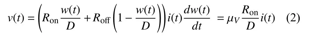
withx(t)∈[0,1]. LetM(t)=Ronx(t)+Roff(1-x(t)). A pinched hysteresis loop figure, the fingerprint characteristic of the memristor, can be obtained by applying a sinusoidal current sourcei(t)=i0sin(ωt) to the memristor. An HSPICE simulation is conducted and the result is shown in Fig. 2. The simulation parameters are set as following:i0= 200 μA,ω=2π rad/s,x(t0)=0.1,t0=0 s,Ron=100Ω,r=Roff/Ron=160,D=10-6cm , µV=10-10cm2/sV.

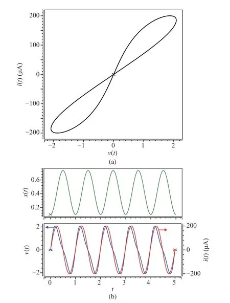
Fig. 2. The dynamical characteristics of the linear HP memristor. (a) The linear memristor’s fingerprint characteristic: pinched hysteresis loop figure.(b) The change of the state x(t) , applied current source i(t) and the corresponding voltage v(t) of the memristor.

Remark 1:From (2) and (3), the memristance is variable in the interval [Ron,Roff]. The memristance will be changed when the voltage or the current source is applied to the device. The initial value of the memristor is the memristancebefore the voltage or the current source is applied. The initial value can be memorized by the memristor and it affects memristance variation. This point, however, has not been discussed in the literature. The simulation parameters are chosen by using those in [3]. We compute the initial state of the memristor with the voltmeterammeter method and consider two cases, i.e., current excitation and voltage excitation, as shown in Fig. 3. The developed methods are for linear and nonlinear dopant drift.

Fig. 3. Circuits for measuring the initial state of a memristor, under the excitation of (a) a current source and (b) a voltage source. V and I are voltmeter and ammeter, respectively.

Let

and

We apply a current source at timet=t0and let

and

Substituting (7) into (3),

and then

Next we verify this method with an HSPICE simulation.Predeterminingx(t0) to be 0.28, we run the circuit in Fig. 3(a)for 2.73 s, while other parameters are the same with those in Fig. 2. The simulation process is presented in Fig. 4. After 2.73 s, the currenti(2.73) and voltagev(2.73) across the memristor are -198.4229 μA and -1.16128 V, respectively.Since the current source is sinusoidal, we getq(2.73)=3.582×10-5C by integratingi(t) fromt=0 tot= 2.73 s. Therefore we can apply the mathematical method and getx(t0)=0.28 which matches the value we predetermined. The result verifies that our method of applying current excitation to determine the initial state of a linear memristor is feasible.

Fig. 4. Simulation process of a linear memristor under the current source for 2.73 s.

B. Linear Dopant Drift With Voltage Excitationthe formula forx(t0) . In (3), let β =D2/µV, and then

In this section, we consider the voltage excitation and drive

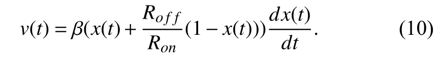
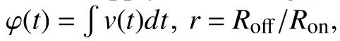
where

It is easy to find that the constantcof the integration is dependent on initial value ofx(t) att=t0. Therefore the memory effect of memristors is attributed to the integration constantc. Next we deduce the analytic expression ofi(t) andv(t). Sincex(t)∈[0,1], from (11), we get

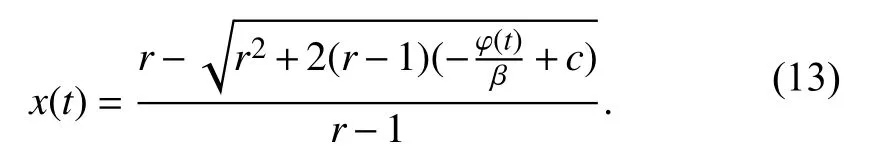
Differentiating (13) with respect to timet, then we obtain

in which constantcis not removed. Based on (3), we have

From (15), we can obtaincby solving (15) withas

Then by (12), the initial statex(t0) can be obtained

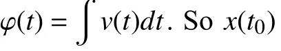
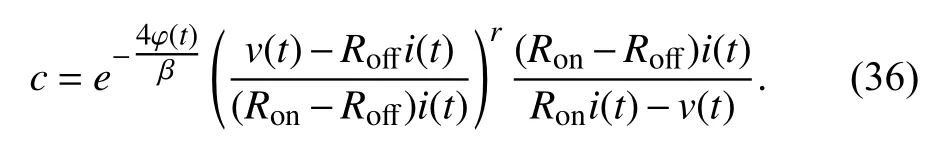
Fig. 5. Simulation process of a linear memristor under the voltage source for 4.21 s.

The result can be easily examined with a simulation. We simulate the circuit Fig. 3(b) on HSPICE. The initial state of the linear memristor is predetermined as 0.37. The applied voltage is a simple sinusoidal voltage sourcev(t)=v0sin(ωt),wherev0=1V, ω =2π rad/s. The other simulation parameters are set as following:t0=0 s,Ron=100Ω,r=160,D=10-6cm, µV=10-10cm2/sV. We run the simulation for 4.21 s. At the end of the simulation, we getv(4.21)=968.5832 mV andi(4.21)=120.7629 μA. Because the applied voltage source is sinusoidal, φ(t) can be calculated from the integration fromt=0 tot=4.21 s: φ(4.21)=0.1196 Wb.Thus we can apply the mathematical method in (17) and obtain

which is the same with what we predetermined forx(t0). From the result, the viability of our method has been examined by the simulation.

C. Nonlinear Dopant Drift With Current Excitation

In this section, we will show the methods to determine the initial statex(t0) of the memristor under the assumption of nonlinear dopant drift. For the nonlinear memristor, the descriptive model should be adjusted from (3) to

wheref(x(t)) is a window function such thatf(0)=f(1)=0 ensures no drift at boundaries. The window function in model(18) is

in whichpis a positive integer.f(x) is shown in Fig. 6 forp=1,2,5, respectively. Aspincreases, the curve get flatter in the middle and becomes steeper at the boundaries. If not specified, all nonlinear memristors are configured asp=1 in the rest of this paper.

Fig. 6. Illustration for window function f(x)=1-(2x-1)2p with p=1,2,5.

Takingp=1 in (19) and combing with (18), we get

The fingerprint characteristic of the memristor with nonlinear dopant drift, a bow-tie shapei-vfigure, can be generated by applying a sinusoidal current sourcei(t)=i0sin(ωt)to the memristor. Based on (20), an HSPICE simulation is performed and the result is shown in Fig 7. The simulation parameters are set as following:i0=800 μA,ω=2π rad/s,r=160,D=10-6cm, µV=10-10cm2/sV.

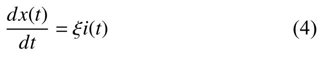
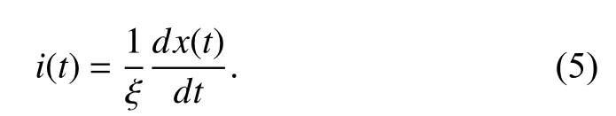
Let ξ =µVRon/D2and simplify (20) as

then

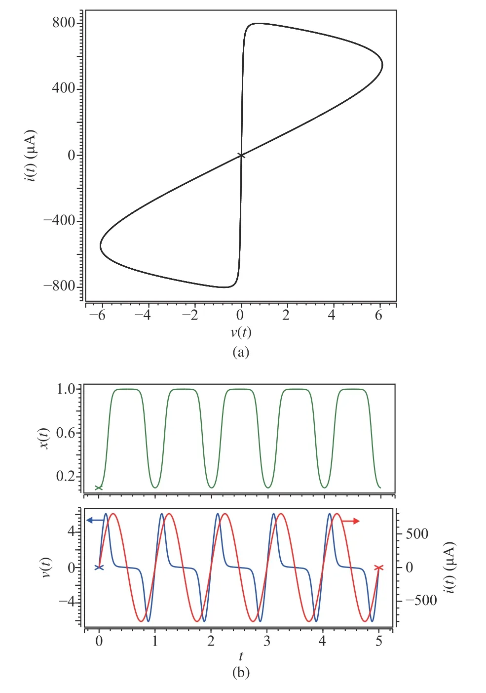
Fig. 7. The dynamical characteristics of the nonlinear HP memristor (a)The nonlinear memristor’s fingerprint characteristic: bow-tie shape figure. (b)The change of the state x(t) , applied current source i(t) and corresponding voltage v(t) of a nonlinear memristor.

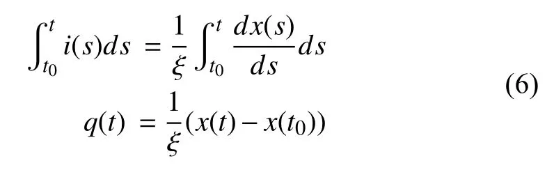
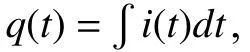
For the initial timet0,q(t0)=0, we integrate both sides of(22) for ∀t＞t0

Let

and solve (23) forx(t), we have

From (24), we can find the determinant relation between the constantcandx(t0). In other words,cincludes the history information ofx(t). Now substitute (25) into (20), and we get

from whichccan be calculated by

Therefore the initial statex(t0) of the nonlinear memristor is obtained by solving (24),

The result of the HSPICE simulation agrees with the method. We presetx(t0)=0.53, and then run the circuit in Fig. 3(a) for 3.67 s. The parameters of the circuit are kept the same with those in Fig. 7. The simulation result is shown in Fig. 8. At the end of the simulation, the currenti(3.67) and voltagev(3.67) of the memristor are - 701.0453 μA and-75.32032 mV, respectively. Because the current source is sinusoidal, we can calculateq(3.67)=1.8866×10-4C by integratingi(t) fromt=0 tot=3.67 s. Therefore

Fig. 8. Simulation process of a nonlinear memristor under the current source for 3.67 s.

The simulation result matches the value we predetermined forx(t0). That means the method is applicable for the calculation of initial states of memristors under the nonlinear dopant drift assumption.

D. Nonlinear Dopant Drift With Voltage Excitation

For nonlinear memristors, the initial statex(t0) can also be acquired through voltage excitation. From (20), we have

where β =D2/µV. Substitutei(t) with (29) into (20), and we get

Let

then (31) can be simplified to

The relation betweencandx(t0) in (32) claims that the initial state of a nonlinear memristor can be calculated from the integration constantc. That is to say, the memory effect of nonlinear memristors can be represented by an integration constant. Next we deduce how to calculatec. Change (33) to

Combining (34) and (35),cis obtained by

Then from (32),x(t0) can be acquired by solving an equation

Since (37) isr-order, whereris undetermined, the analytical solution ofx(t0) is not easy to get. So a numerical solution is recommended.

In order to get the numerical solution ofx(t0), an algorithm is presented as follows. First, construct a functionz(x)according to (37)

Forx(t0)∈(0,1) , iteratex(t0) from 0 to 1, with a small increment δ (e.g., δ =0.0001) in each iteration. Notice that the precision of the numerical solution is dependent on δ: the smaller δ, the better the accuracy. During the iteration,x(t0) is regarded as the independent variablexto calculatez(x) in(38). Since the derivative ofz(x)

z(x) is monotonically increasing with the increment ofxin every step. Continue the iteration until obtaining asuch thatthen compare the absolute value ofandto select the smaller one. As a result, the correspondingxto this smallerz(x) is the numerical solution ofx(t0) we are looking for.

An HSPICE simulation is conducted to verify this approach.The simulation circuit is the same with Fig. 3(b).Predetermining the initial state of the nonlinear memristor as 0.41, we apply a simple sinusoidal voltage sourcev(t)=v0sin(ωt) , wherev0=1.2 V, ω=2π rad/s. The other simulation parameters are set as following:t0=0 s,Ron=100 Ω,r=160,D=10-6cm, µV=10-10cm2/sV. The simulation lasted for 3.73 s and we getv(3.73)=-1.190538 V andi(3.73)=-243.4537 μA. Since the applied voltage source is sinusoidal, φ(t) can be calculated from the integration fromt=0 tot=3.73 s: φ(3.73)=0.2149 Wb. Thus we can apply our mathematical method in (36)-(38) and obtain

The calculation result ofx(t0) is the same with what we predetermined. The feasibility of our method has been examined from the simulation.Remark 2:From the analysis above, the integration constantcincludes the information of the initial valuex(t0). The memory is attributed to the integration constantc, which means that the initial valuex(t0) can be computed by the integration constantc. For different models of the memristors,the formulas of the integration constantcare different. The accuracy of the initial value computation is dependent on the model of the device.

E. Memory Analysis for MRNNs

The model of the MRNNs is obtained by replacing linear resistors with memristors and can be described by the following differential systems

Fig. 9. Simulation process of a nonlinear memristor under the voltage source for 3.73 s.

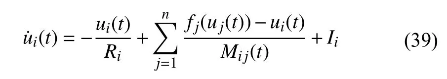
whereui(t),i=1,2,...,n, are the states of the network,Ri,Mij(t),i,j=1,2,...,n, are linear resistances and memristances, respectively;fj(s) andIi,i,j=1,2,...,n,s∈R are activation functions and bias currents, respectively.

According to the property of memristor, MRNNs are a cluster of neural networks. When the power is off, MRNNs can store their historic state. In order to analyze their memory property, i.e., computing initial values of every memristors,we use Algorithm 1 for the memory analysis for MRNNs.

Algorithm 1 Memory analysis for MRNNS

Remark 3:From (39), coefficients of MRNN are variable in the interval [ 1/Roff,1/Ron]. If the MRNN can be convergent to one sub-network, the convergent result is dependent on the initial valueui(t0) of the network state and the initial valueMji(t0)of memristive synapses. It is necessary for us to locate the initial state of memristive synapses, i.e., analyzing the memory property of the memristor. It is difficult to obtain an accurate value of the voltage between two terminals of memristors. In future works, we will design suitable observers to obtain the voltage value of memristors. Memristors are nano-scale nonlinear resistors with stationaryRonandRoff. In practical applications, we need to connect two or more memristors in series or parallel to obtain different memristors with different memristances. Therefore, it is necessary to analyze the memory of two or more memristors in series or parallel.

III. MEMORY PROPERTIES OF TWO MEMRISTORS INTERCONNECTION

In this section, we will discuss memory properties of two series and parallel memristors. As discussed in Section II, one measurement value (i(t) orv(t)) and one integration value (q(t)or φ(t)) is needed to determine the initial state of the memristor. However, we do not need to conduct two measurements and two integrations for two memristors when they are connected in series or parallel, because the memristors connected in series share the same current, and the ones in parallel share the same voltage. Our approach is valid forn(n＞1) memristors connected in series and parallel: for the series connection case,nmeasurements fornindividual voltages and an integration for the common charge are required; for the parallel connection case, we neednmeasurements fornindividual currents and an integration for the shared magnetic flux. For the purpose of simplicity and without loss of generality, we only discuss two series and parallel memristors.

A. Two Memristors in Series

Firstly we discuss the memory property of two memristorsM1andM2in series and discuss the method in finding initial states ofM1andM2. Denotex1(t0),x2(t0) as initial states ofM1andM2. Then one can attach a given current sourcei(t) to them and measure the corresponding voltagev1(t),v2(t)ofM1,M2. When two memristors are connected in series, we should consider the memristors’ polarities as shown in Fig. 10. In the situation of Fig. 10(a),M1andM2connected in series share the same polarity with the current source and voltmeters. We can directly apply (28) in Section II to each memristor. In Fig. 10(b), whileM1shares the same polarity with the excitation,M2is opposite to the current source. Hence calculation methods for the initial state ofM2should be adjusted. A negative sign should be added toi(t),v(t) andq(t)to offset the polarity difference ofM2. Since the existence of opposite polarity is more universal for series connected memristors, in this subsection, we only discuss the situation in Fig. 10(b).

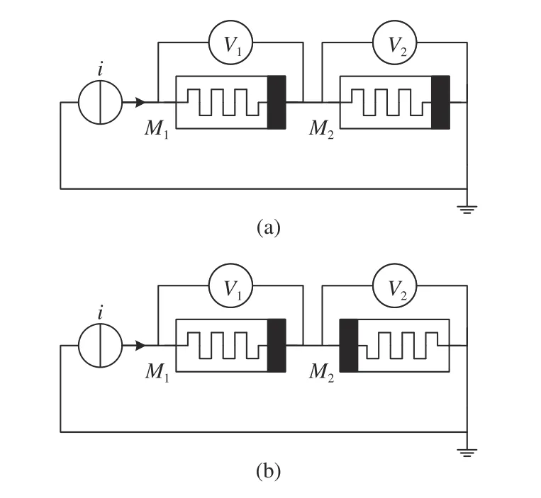
Fig. 10. Two memristors in series with (a) the same polarity and (b) the opposite polarity.

If the discussed memristors are under the assumption of linear dopant drift, we calculate the integration constantc1and the initial statex1(t0) ofM1. ForM2, the memristor opposite to the one connected,

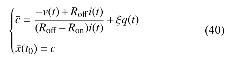
An HSPICE simulation is conducted to examine this method for linear memristors in series. We predetermine the initial statesx1(t0),x2(t0) to be 0.15 and 0.75, respectively.The simulation circuit is Fig. 10(b), where the current sourcei(t)=i0sin(ωt),i0=200 μA , and ω=2π rad/s. The other simulation parameters are the same as the ones in Section II:t0=0 s,Ron=100 Ω,r=160,D=10-6cm, µV=10-10cm2/sV.We then run the circuit for 3.13 s.i(3.13)=145.7937 μA,v1(3.13) andv2(3.13) are measured as 1.752215 V and 826.8759 mV, respectively. Since the current source is sinusoidal, we getq(3.13)=1.0041×10-5Cby integratingi(t)fromt=0 tot=3.13 s. With the presence ofi(3.13),vk(3.13)andq(3.13),k=1,2, the initial states ofM1,M2are obtained according to (40),

The results are coincident with the values we preset forx1(t0),x2(t0), representing the validity of the methods (40).

For series connected memristors under the assumption of nonlinear dopant drift, the integration constantc1and the initial statex1(t0) ofM1can be calculated from (28). As for the opposite connectedM2, (28) should be adjusted to

Hencec2andx2(t0)ofM2can be obtained from (41).

This approach for series connected memristors with the nonlinear dopant drift can also be verified with an HSPICE simulation. We preset the initial statesx1(t0),x2(t0) to be 0.21 and 0.47, respectively. The simulation circuit and parameters are identical to the ones above for linear memristors, except the magnitude of the current source isi0=800 μA. Run the circuit for 4.11 s. At the end of the simulation,i(4.11)=509.9392 μA,v1(4.11) andv2(4.11) are measured as 4.420901 V and 6.407382 V, respectively. Since the current source is sinusoidal, we can getq(4.11)=2.9219×10-5C by integratingi(t) fromt=0 tot=4.11 s. Now we havei(4.11),vk(4.11) andq(4.11),k=1,2, the initial states ofM1,M2can be calculated according to (28) and (41)

The predetermined values forx1(t0),x2(t0) are obtained from the simulation, showing the feasibility of methods (28)and (41).

B. Two Memristors in Parallel

In this subsection, we study the property of two memristors in parallel and give the formulas to calculate the initial states ofM1,M2. A common voltage sourcev(t) is applied to them and the corresponding currentsi1(t),i2(t) ofM1,M2can be measured. When two memristors are connected in parallel, we should consider the memristors’ polarities as shown in Fig. 11.In Fig. 11(a),M1andM2connected in parallel share the same polarity with the voltage source and the ammeters. Equations(17) or (36), and (37) in Section II can be applied to each memristor. In Fig. 11(b) , however,M2is opposite to the voltage excitation, contrary to the regular connection ofM1.Therefore the calculation methods for the initial state ofM2should be adjusted accordingly. A negative sign is added tov(t),i(t) and φ(t) to compensate for the polarity difference ofM2. We only discuss the situation in Fig. 11(b) in this subsection, because the existence of opposite polarity is more general for parallel connected memristors.

First we discuss the memristors in parallel under the linear dopant drift assumption; the integration constantc1and the initial statex1(t0)ofM1can be calculated from (17). Whilec2andx2(t0) of the opposite connected memristorM2can be obtained

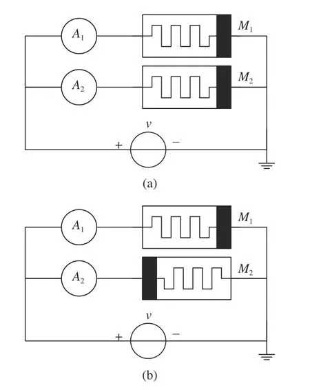
Fig. 11. Two memristors in parallel with (a) the same polarity and (b) the opposite polarity.

A parallel memristors circuit simulation is conducted to examine this method. We preset the initial statesx1(t0),x2(t0)to be 0.33 and 0.67, respectively. The simulation circuit is in Fig. 11(b), where the applied voltage is a simple sinusoidal voltage sourcev(t)=v0sin(ωt),v0=1 V, ω=2π rad/s. The other simulation parameters are the same with those in series connection. Run the simulation for 5.21 s. Thenv(5.21)=968.5831 mV,i1(5.21) andi2(5.21) are measured as 109.9511 μA and 118.6726 μA, respectively. We can also get φ(5.21)=0.1196 Wb by integratingv(t) fromt=0 tot=5.21s since the voltage source is sinusoidal. With the existence ofv(5.21),ik(5.21) and φ(5.21),k=1,2, the initial states ofM1,M2are obtained according to (17) and (42),c1=-44.1424,x1(t0)=0.33,c2=-71.5125,x2(t0)=0.67.

The correctness of our approach is examined from the consistency of the result and preset values.

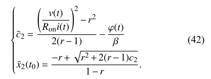
Then we should consider the situation when two memristors under the assumption of nonlinear dopant drift are connected in parallel. The integration constantc1ofM1can be calculated from (36), and the initial statex1(t0) can be obtained from solving (37). The numerical algorithm to determine the solution of (37) has been described in Section II-D. As for the opposite connectedM2, (36) should be adjusted to

to get the integration constantc2ofM2. Andx2(t0), the initial state ofM2, can also be obtained from solving the equation

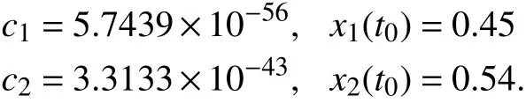
We simulate the nonlinear memristors in parallel to test this algorithm. Predetermining the initial statesx1(t0),x2(t0) to be 0.45 and 0.54, respectively. The circuit and parameters are the same with the previous ones, except the magnitude of the voltage sourcev0=1.2 V. The simulation is lasted for 5.77 s.At the end of the simulation,v(5.77)=-1.190538 V,i1(5.77)andi2(5.77) are measured as - 230.0400 μA and-115.2139 μA, respectively. Since the voltage source is sinusoidal, we can calculate φ(5.77)=0.1670 Wb by integratingv(t) fromt=0 tot=5.77 s. Now we getv(5.77),ik(5.77) and φ(5.77),k=1,2, the initial states ofM1,M2can be obtained following the calculation of (36), (43) and the solution of (37), (44),

The results are in accordance with the predetermined values.

Remark 4:For two memristors connected in series or parallel, the total initial memristance can be computed if the initial valuesx1(t0),x2(t0) are obtained, respectively. We focus on the memory analysis for two memristors in series or parallel, i.e., the total initial memristance computation. This is difference from the property analysis of two series or paprallel memristors in the existing papers.

IV. CONCLUDING REMARKS

In this paper, we discuss the memory property of memristors by deriving the formula for the initial value formula and the voltmeter-ammeter method. Then we analyze two series and parallel memristors' memory. According to the developed memory analysis method, we give the algorithm for locating the initial values of all memristive synapses of the MRNN (39). Our analysis shows that the integration constantcin the expression plays an important role in the memory of the electronic device. The accuracy may be improved for the computation of the initial values if the state observer can be designed for the MRNN. This will be our future work.