YANG Wensheng(杨文生)ZHENG Yanhong(郑艳红)

( 1.College of Mathematics and Informatics,Fujian Normal University,Fuzhou 350007,China; 2.FJKLMAA,Fujian Normal University,Fuzhou 350007,China)

Abstract: A stage structure predator-prey model with prey refuge and Beddington-DeAngelis functional response is considered in this work.The sufficient condition which ensures persistence of the system is obtained by using a comparison method.Furthermore,the sufficient conditions for the global asymptotical stability of the unique positive equilibrium of the system are derived by constructing suitable Lyapunov function.It is shown that our result supplements and complements one of the main results of Khajanchi and Banerjee (2017).

Key words: Stage structure; Prey refuge; Beddington-DeAngelis functional response;Persistence; Global asymptotical stability

1.Introduction

In [1],Khajanchi and Banerjee studied the following predator-prey model with stage structure and ratio-dependent functional response

wherexi(t),xm(t) andy(t) are the densities of immature/juvenile preys,mature/adult preys and predators at timetrespectively.αrepresents the growth rate of immature preys.The conversion coefficient from juvenile preys to adult preys is proportional to the existing juvenile preys with proportionality constantβ.δ1,δ2andδ3are the natural death rates of juvenile preys,adult preys and predators,respectively.γrepresents the intra-species competition(overcrowding) rate of adult preys.They introduced a refugeθxm(t),of the adult preys(θ ∈(0,1)),which measures the degree or strength of prey refuge.(1−θ)xm(t) is the density of adult preys available to predators for their foods/nutrients.The predator population captures the adult preys following ratio-dependent functional responseTherepresents the conversion of nutrients into the reproduction of predators.They also assumed that the juvenile preys are not accessible to predators as they are highly protected and kept out of reach by their parents.For more biological background of system(1.1),one could refer to [1] and the references cited therein.

As we know,ratio-dependent predator-prey models have been introduced and studied extensively [2-4].However,it has somewhat singular behavior at low densities and has been criticized on other grounds.See [3] for a mathematical analysis and the references in [2]for some aspects of the debate among biologists about ratio dependence.The Beddington-DeAngelis form of functional response has some of the same qualitative features as the ratiodependent form,but avoids some of the behaviors of ratio-dependent models at low densities which have been the source of controversy.For more biological background of the model with Beddington-DeAngelis functional response,one could refer to [5-8].

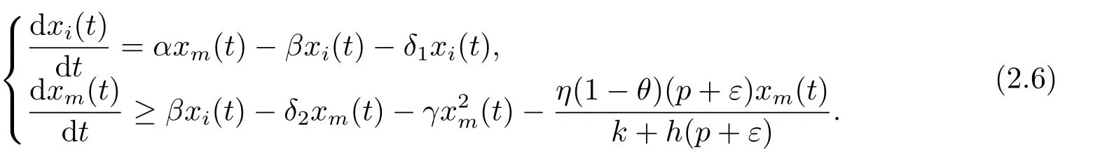
Motivated by the above study,we are interested in considering system(1.1)with Beddington-DeAngelis functional response,

wherexi(t),xm(t) andy(t) are the densities of immature/juvenile preys,mature/adult preys and predators at timetrespectively.We assume that functional response is of Beddington-DeAngelis functional response,that is

wherekdenotes the saturation constant.In fact,letk=0,then the system (1.2) can be transformed to the system (1.1).Therefore,lettingk →0,we can see more dynamical behaviors of the system (1.1) clearly by studying the system (1.2).

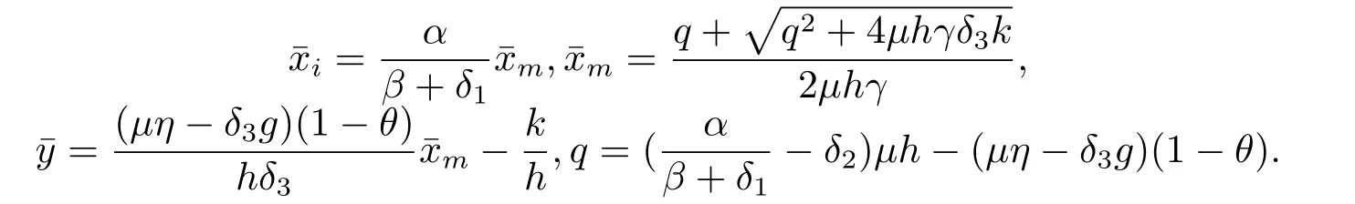
It is easy to verify that the system (1.1) has a unique positive interior equilibriumE∗(x∗i,x∗m,y∗),if and only if

and

hold,where

In [1],Khajanchi and Banerjee obtained sufficient conditions for the uniform persistence and global asymptotic stability,that is,they obtained the following results.

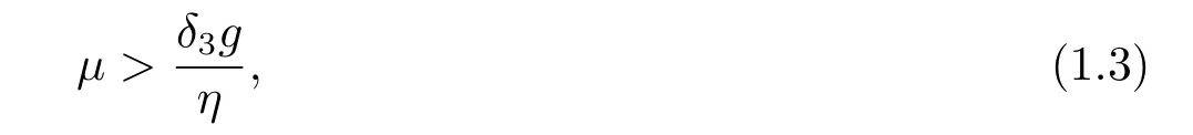
Theorem AIf (1.3) holds,then system (1.1) is uniformly persistent.

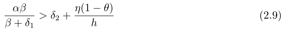
Theorem BThe positive interior equilibrium pointE∗(x∗i,x∗m,y∗)of(1.1),with positive initial conditionxi(0)>0,xm(0)>0,y(0)>0,is globally asymptotically stable if (1.3) and

hold.

However,we should point out that the condition (1.3) is not sufficient for persistence of the system (1.1) in Theorem A.Firstly,we will give a definition of persistence of the system(1.1).

Definition 1.1The system (1.1) is said to be persistent if for any nonnegative initial data (xi(0),xm(0),y(0)) withxi(0)>0,xm(0)>0,y(0)>0,there exist positive constantsϵ1,ϵ2,ϵ3such that the solution (xi(t),xm(t),y(t)) of (1.1) satisfies

Now,we show that the condition (1.3) is not sufficient for persistence of the system (1.1) in Theorem A.In fact,in the process of the proof of Theorem A in [1],Khajanchi and Banerjee obtained that

Obviously,under the condition (1.3),one can’t obtainϵi>0,i=1,2,3.

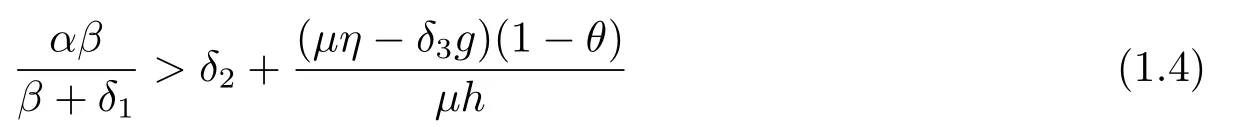
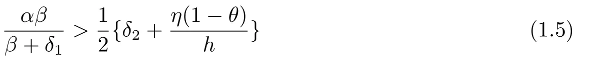
Similarly,we should also point out that the conditions (1.3) and (1.5) are not sufficient for global asymptotical stability of the positive equilibrium pointE∗(x∗i,x∗m,y∗) of system(1.1) in Theorem B.To show this,we will give an example.Let us takeα=1.0,β=0.25,δ1=0.03,δ2=0.125,δ3=0.4,γ=2.1,η=3.0,g=0.9,h=1.0,µ=0.5,θ=0.5.Thus,µη=1.5,δ3g=0.36,Obviously,µη > δ3g,that is,the conditions(1.3) and (1.5) hold,but the condition (1.4) doesn’t hold.Unfortunately,the conditions(1.3) and (1.5) are not enough to ensure that there is a unique positive interior equilibriumE∗(x∗i,x∗m,y∗) of the system (1.1),much less to prove global asymptotical stability of the positive equilibrium.

As well known,the persistence and the global stability are two important topics in the study of dynamics for differential equations and population models.In the present article,we shall also concern with these two topics,that is,we will prove a new persistent property and global stability result for the system (1.1) and (1.2) by using a comparison method and constructing suitable Lyapunov function respectively,and our result significantly improves and supplements the earlier one given in[1].The rest of this paper is organized as follows.In Section 2,we investigate the persistence property of the systems (1.1) and (1.2).In Section 3,we will discuss global stability of the positive equilibrium point of the systems (1.1) and(1.2).In Section 4,the conclusion and discussion are given in the end of this paper.

2.Persistent Property

In this section,we will show that any nonnegative solution(xi(t),xm(t),y(t))of(1.2)lies in a certain bounded region ast →+∞.From the viewpoint of biology,this implies that the immature prey,mature prey and predators will always coexist at any time.

Theorem 2.1If (1.3) and

hold,then system (1.2) is uniformly persistent,where

ProofLet (xi(t),xm(t),y(t)) be any positive solution of system (1.2).From the first two equations of system (1.2),we have

Consider the following comparison system

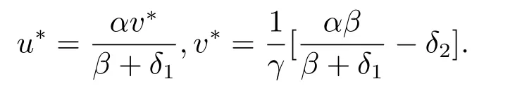
It is easy to know that there are a bound equilibrium (0,0) and a unique positive equilibrium(u∗,v∗) of the system (2.3),where

Define a Lyapunov function of (2.3) as follows:

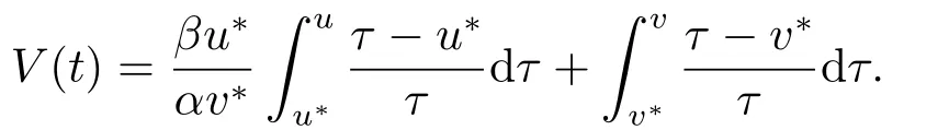
It is easy to see thatV(t)>0 as (u,v)(u∗,v∗).Calculating the derivative along the solutions of (2.3),we obtain

and the equality holds only whenu=u∗,v=v∗.By LaSalle’s invariance principle[9],it follows that (u∗,v∗) is globally asymptotically stable.

Thus,there existsT1>0 such that ift ≥T1,u(t)≤u∗+ε,v(t)≤v∗+ε(whereε >0 is very small).Letxi(T1)=u(T1),xm(T1)=v(T1).Standard comparison argument indicates that

From the third equation of (1.2)and (2.4),we have

fort>T1.By comparison theorem,for the aboveε>0,there is aT2>T1,such that

Consider the following comparison system

It is easy to know that there are a bound equilibrium (0,0) and a unique positive equilibrium(u∗1,v∗1) of the system (2.7),where

By using the same proof as in the step (2.3),one can show that for the aboveε >0,there is aT3>T2,such that for anyt ≥T3,

From (2.8) and (2.1),we can easily obtain that

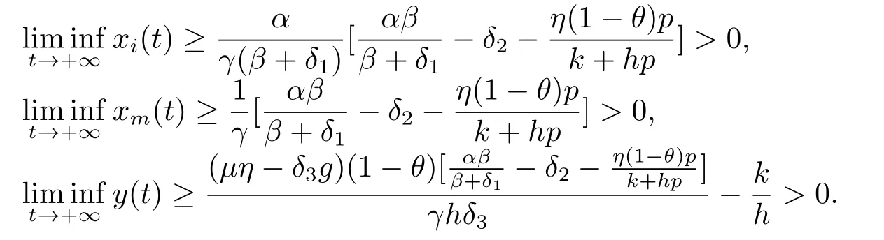
From Definition 1.1,we can easily obtain that the system (1.2) is uniformly persistent.The proof is complete.

Letk=0,then the system (1.2) can be transformed to the system (1.1).Therefore,we obtain the following theorem.

Theorem 2.2If (1.3) and

hold,then the system (1.1) is uniformly persistent.

3.Global Asymptotical Stability

The following lemma describes the existence of a unique positive equilibrium of model(1.2).

Lemma 3.1If (1.3) and

hold,then there exists a unique positive equilibriumwhere

ProofLemma 3.1 can be proved by simple direct calculation,thus it is omitted here.

From the viewpoint of ecology,the constant positive steady-state solution implies the coexistence of the immature prey,mature prey and predators.Now,we will discuss the global stability of the positive equilibriumfor the system (1.2).

Theorem 3.1The positive interior equilibrium pointof the system (1.2)is globally asymptotically stable if (1.3) and

hold.

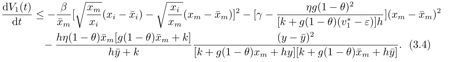
ProofLet (xi(t),xm(t),y(t)) be a positive solution of (1.2).To prove our statement,it suffices to construct a Lyapunov function.For this purpose,we define

From (2.8),for anyt>T3,xm(t)≥v∗1−ε.Hence,for anyt>T3,we have

From (3.2),we can easily obtain that for above sufficiently smallε>0,

It follows from (3.5) that

and the equality holds only whenBy LaSalle’s invariance principle[9],it follows thatis globally asymptotically stable.

Letk=0,then the system (1.2) can be transformed to the system (1.1).Therefore,we can also obtain the following theorem.

Theorem 3.2The positive interior equilibrium pointE∗(x∗i,x∗m,y∗)of the system(1.1)is globally asymptotically sta ble if (1.3) and

hold.

4.Conclusion and Discussion

In this paper,a stage structure predator-prey model with prey refuge and Beddington-DeAngelis functional response is investigated.On one hand,we achieve sufficient conditions of the persistence of the systems(1.1)and(1.2).On the other hand,we analyze global asymptotical stability of the positive interior equilibrium point by constructing suitable Lyapunov function.

In[1],Khajanchi and Banerjee also discussed the sufficient conditions for the persistence and global asymptotical stability of the system (1.1),but the conditions which they obtained are not sufficient (see Section 1).However,why can they obtain the results of the persistence and global asymptotical stability of the system (1.1) by numerical simulation? In fact,the parameter values in their numerical simulation fortunately satisfy the conditions of Theorem 2.2 and Theorem 3.2.Therefore,they obtain correct numerical results.However,if they numerically simulate the model (1.1) for the set of other parameter values in the region of conditions of Theorem 3 and Theorem 4 in[1],then they may not obtain the correct numerical results.It is shown that our result supplements and complements one of the main results of Khajanchi and Banerjee[1].