Haoshu Shen,Yuxin Wu, *,Minmin Zhou,Hai Zhang,Guangxi Yue

1 Key Laboratory for Thermal Science and Power Engineering of Ministry Education,Department of Energy and Power Engineering,Tsinghua University,Beijing 100084,China

2 Institute for Clean and Secure Energy,Department of Chemical Engineering,University of Utah,Salt Lake City 84112,United States

Keywords:Particle dispersion Subgrid-scale modeling Forced isotropic turbulence Stokes number

ABSTRACT The subgrid-scale effects on particle motion were investigated in forced isotropic turbulence by DNS and prior-LES methods.In the DNS field,the importance of Kolmogorov scaling to preferential accumulation was validated by comparing the radial distribution functions under various particle Stokes numbers.The prior-LES fields were generated by filtering the DNS data.The subgrid-scale Stokes number(StSGS)is a useful tool for determining the effects of subgrid-scale eddies on particle motion.The subgrid-scale eddies tend to accumulate particles with StSGS＜1 and disperse particles with 1＜StSGS＜10.For particles with StSGS≫1,the effects of subgrid-scale eddies on particle motion can be neglected.In order to restore the subgrid-scale effects,the Langevin-type stochastic model with optimized parameters was adopted in this study.This model is effective for the particles with StSGS＞1 while has an adverse impact on the particles with StSGS＜1.The results show that the Langevin-type stochastic model tends to smooth the particle distribution in the isotropic turbulence.

1.Introduction

Gas-solid two phase flows are widely applied to many industrial applications.Besides experimental studies,computational fluid dynamics(CFD)is a useful tool to investigate the flow mechanisms.CFD methods can be classified as Reynolds-Averaged Navier-Stokes(RANS)simulation,large eddy simulation(LES)and direct numerical simulation(DNS)[1].DNS resolves all the turbulent scales in the flow fields.However,the tremendous computational costs impede its industrial applications.LES explicitly calculates large-scale eddies and models subgridscale(SGS)eddies in the flow fields.Apte et al.concluded that LES was more accurate than RANS when predicting the turbulent mixing and particle dispersion[2].The SGS effects on particle motion in LES have attracted a great deal of attention in recent years.It may improve the prediction accuracy of particle-laden turbulent flows which are widely employed in lots of engineering devices such as engines and furnaces.Yeh and Lei found that the particle motion was controlled mainly by the large eddies and the effects of small eddies could be neglected[3].Yang and Lei concluded that the phenomenon of particle accumulation in the low vorticity region was mainly controlled by the small scales with wavenumber kωcorresponding to the maximum of the dissipation spectrum[4].Armenio et al.showed that the SGS eddies affected particle dispersion significantly only when the filter width was large or the particle inertia was small[5].However,the aforementioned studies failed to propose any dimensionless quantities to determine in which circumstances the SGS eddies were important to the particle motion.Fede and Simonin proposed a ratio of the mean particle response time to the subgrid Lagrangian integral time seen by the particles[6].Marchioli et al.plotted the particle segregation parameter with the Stokes number based on Kolmogorov time scales in turbulent channel flows[7].Urzay et al.analyzed the particle-laden turbulent flows theoretically by defining a SGS Stokes number in LES[8].Thus,it is necessary to assess the performance of this quantitative index when tracking particles in the LES flow fields.

The second issue relates to how to reconstruct the SGS effects on particle motion.The stochastic models based on the Langevin equation were originally proposed for modeling the turbulent dispersion of particles in RANS[9,10].Fede et al.derived the general form of the Langevin equation along inertial particle trajectories in LES[11].This model was assessed in priori and posteriori tests and was proved effective in some scenarios[12-14].It is worth mentioning that there are two undetermined parameters which may affect the model performance.They are the Lagrangian SGS fluid velocity time scale(δTLp)and the fluid SGS kinetic energy(kSGS,p)seen by an inertial particle.Wang and Stock proposed an empirical equation of the fluid time scale seen by a heavy particle of zero drift[15].Fede and Simonin have shown that the Wang and Stock's model gave poor predictions for the intermediate Stokes number[6].Some researchers simply assumed that δTLpand kSGS,pcould be modeled by the fluid SGS properties[12,14]or full-scale properties[13].Jin et al.fitted the DNS data by an empirical curve which was superior to the Wang and Stock's model[16,17].The effects of the optimized model parameters on particle motion should be evaluated under various particle Stokes numbers.

This paper investigated the particle motion influenced by SGS eddies in a forced isotropic flow.The LES flow fields were generated by filtering the DNS data with different filter sizes.The effects of SGS turbulence on particle motion were evaluated from the perspective of SGS Stokes number.The performance of the Langevin-type stochastic model with improved parameters was studied under various particle Stokes numbers.

2.Fluid Simulations

2.1.DNS database

The DNS data of the forced isotropic turbulence were obtained from the Johns Hopkins Turbulence Databases[18].In consideration of the storage capacity,only a small portion of the DNS data were extracted from the database.The simulation domain was a cube with a side length of π/8.There were 64 nodes uniformly distributed on each side.The simulation time-step was 0.0002 and the data was stored every 10 time-steps over a time period of 1.The fluid viscosity was set as 0.000185.The statistical charateristics of turbulence were shown in Table 1.

2.2.Filtered DNS fields

The DNS fields were filtered by the box filters of different sizes to generate the prior-LES fields.The filtered quantity f is defined as:

where F is the box filter.This filter shown in Eq.(2)corresponds to an averaging over a cubic box of size λ[1].

The filter sizes were chosen as 2Δ,4Δ,8Δ and 16Δ where Δ(Δ=π/512)denoted the mesh size of the DNS field.The ratios of the resolved turbulent kinetic energy to the full-scale turbulent kinetic energy were 0.95,0.89,0.77 and 0.59 respectively.Fig.1 compared the energy spectrums of DNS and prior-LES fields.It showed that the cut-off wave number decreased with the increased filter size.

Fig.1.Turbulent energy spectrums of the DNS and prior-LES fields.

Table 1 Statistical characteristics of turbulence

3.Particle Tracking in the Flow Fields

3.1.Single particle motion equation

The ratio between particle and fluid densities is much larger than 1.Thus,all forces except the drag and gravity forces can be neglected[6].The aim of this paper is to investigate the effects of SGS eddies on particle motion,so the gravity force is not included in the equation for the sake of simplicity.The single particle motion equation is finally reduced to:

where the subscript g denotes the gas phase,p denotes the particle phase and τpis the particle relaxation time.fdragis the coefficient of the drag force and can be expressed as a function of the particle Reynolds number(Rep)[19].

3.2.Stochastic modeling of subgrid-scale effects

The Langevin-type stochastic equation was adopted to capture the SGS velocities(ui∗)seen by particles along their trajectories[11]:

where dWiis an increment of the Wiener process[20].The gradients of the residual stress tensors and filtered velocities on the RHS of Eq.(7)could be neglected in the isotropic turbulence[14].δTLpand kSGS,p,which vary with the filter size and particle Stokes number,are needed to be optimized in the simulations.Jin et al.introduced an empiricalconstant to relate kSGS,pto kSGS[16]:

Table 2 Particle Stokes numbers of DNS and LES flow fields

Fig.2.RDF of particles distributed in the DNS field:(a)10-30 μm and(b)30-200 μm.

where kSGSis the fluid SGS kinetic energy averaged over the whole space and C0depends on the Stokes number scaled by Kolmogorov timescale.When the Stokes number is very large or very small,C0tends to approach 1.When the Stokes number is near 1,kSGS,pis usually lower than kSGS.However,Pozorski and Apte set C0=1 regardless of the Stokes number[14].kSGScan be defined from the residual-stress tensor τij[21]:

where uiis the component of fluid velocities.

Fig.3.Instantaneous particle distributions in the DNS field:(a)10 μm,(b)30 μm,(c)40 μm and(d)200 μm.

Jin et al.improved the prediction of δTLpby fitting the DNS data with an empirical curve[16]:

where βδ=δTL/δTE,St=τp/δTE,kcf=π/Δ and η is the Kolmogorov length scale.This equation was verified by the DNS results when ηkcf=0.135.According to the equation,δTLpapproaches δTLfor small Stokes numbers while approaches δTEfor large Stokes numbers.These findings were consistent with theoretical analysis.

The crossing-trajectory effect was also taken into account by extending the model for RANS particle dispersion to LES[10,12].The SGS time scale should be adjusted for the directions parallel and perpendicular to the relative velocity of fluid and particle phases.

where β=TL/TEandYeung found that β=0.72 was insensitive to the Reynolds number in stationary isotropic turbulence[22].A discrete form of the Langevin equation was adopted in the simulations[14].

Fig.4.Comparison of RDF for DNS and LES:(a)20 μm,(b)30 μm,(c)40 μm,(d)57 μm,(e)100 μm and(f)200 μm.

where Δt is the time interval and ξiare Gaussian random numbers generated ateach time step.Eq.(14)was unconditionally stable and had the first-order accuracy in time.Lemons provided detailed information on how to solve the Langevin equation[20].

3.3.Particle settings

The particle diameters were set as 10×10-6,2 0×10-6,3 0×10-6,40×10-6,57×10-6,1 0 0×10-6,2 0 0×10-6respectively.The ratio of the particle density to the fluid density was around 68931.35937(333)particles were uniformly distributed in the simulation domainat the initial time step.The time interval of the simulation was 0.002 s,which was larger than the parti-cle relaxation time.The assumption ofone-way coupling was adopted for the fluid-particle interaction.In prior-LES simulations,the filtered fluid velocities interpolated at the particle location were used in Eq.(3).In order to account for the SGS effects,the SGS velocities seen by particles were added to the filtered fluid velocities.

Table 1showed the Kolmogorov-scale and SGS Stokes numbers of particles in DNS and LES flow fields.The particle Stokes number is important for evaluating the effects of SGS eddies on particle dispersion.For StSGS≫1,the effects of SGS eddies can be neglected.For StSGS=1,the particles tend to closely follow the SGS eddies.For StSGS～1,the effects of SGS eddies should be taken into account.All the three regions determined by the SGS Stokes number were covered in each LES flow field.The cut-off location was at ηkcf=0.128 when the filter width was 8Δ.It was close to the LES field studied by Jin et al[16].Thus,the stochastic dispersion model was only evaluated in the LES field with the filter width of 8Δ.The last column in Table 2 has shown that the model constant C0of kSGS,pvaried with the Kolmogorov-scale Stokes number.

Fig.5.Comparison of RDF for DNS,LES without SGS dispersion model and LES with the model:(a)20 μm,(b)30 μm,(c)40 μm,(d)57 μm,(e)100 μm and(f)200 μm.

4.Results and Discussions

4.1.Quantification of preferential concentration

The preferential concentration of particles can be quantified by the radial distribution function(RDF)[23].The two-particle jointprobability function is defined as:

where P（N）（）represents the joint probability that each particle in the domain lies within volumes…,throughThe two-particle RDF can be derived from Eq.(17):

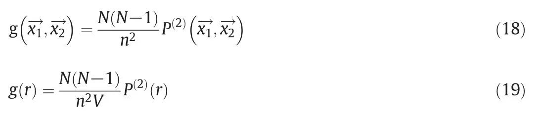
Fig.6.Instantaneous particle distributions for 30 μm particles(StSGS=0.55):(a)DNS,(b)LES without the SGS dispersion model,(c)LES with the model.

where N is the number of particles,V is the volume and n=N/V is the particle number density.For a statistically isotropic and homogeneous system of particles,RDF can be expressed in terms of the relative separation distanceg(r)equals to 1 for uniformly distributed particle systems and is larger than 1 for particle systems featuring the preferential concentration.

4.2.Particle dispersion in the DNS field

Particle dispersion was first analyzed in the DNS field in order to verify the Kolmogorov scaling criterion.Fig.2 plotted RDF versus the dimensionless separation distance normalized by the Kolmogorov scale.RDF went down dramatically and then approached unity as r/η increased.It meant that the particle preferential concentration was likely to be influenced by small turbulent scales.The Kolmogorov-scale Stokes numbers for the chosen particles ranged from 0.10 to 38.65.Fig.2 showed that RDF increased as Stkchanged from 0.10 to 0.90 while declined as Stkchanged from 0.90 to 38.65.The maximum value of RDF appeared when Stkwas near 1.The results were consistent with the Kolmogorov scaling criterion.

Fig.3 compared the instantaneous particle distributions in the DNS field.When Stkwas much smaller or larger than 1(Fig.3a and d),the particles tended to be fully dispersed in the simulation domain.When Stkwas near 1(Fig.3b and c),the particles were significantly concentrated in certain regions.The Kolmogorov scales played an important role on particle transport in the DNS field.

4.3.Particle dispersion in the LES field

Since the unresolved turbulent kinetic energy was significant for large filters(8Δ and 16Δ),the effects of SGS eddies on particle motion couldn't be neglected.The particle distributions of LES fields were compared to those of DNS fields in Fig.4.The SGS Stokes numbers were less than 1 when the particle size was below 57 μm for the LES fields with filter sizes of 8Δ and 16Δ.In Fig.4(a)-(c),the RDFs of LES fields were lower than those of DNS fields.The particles(StSGS＜1)tended to be dispersed when neglecting the SGS eddies.In Fig.4(d)and(e),the RDFs of LES fields were larger than those of DNS fields.The particle distributions(1＜StSGS＜10)were more concentrated without modeling the SGS effects on particle motion.Fig.4(f)presented that the SGS eddies had little effects on particle distributions when StSGS≫1.The SGS Stokes number was a useful tool for determining whether or not the particle dispersion on subgrid scales should be considered.For small SGS Stokes numbers(StSGS＜1),the preferential concentration was enhanced by SGS eddies.For intermediate SGS Stokes numbers(1＜StSGS＜10),the SGS eddies tended to randomize the particle motion.For large SGS Stokes numbers(StSGS≫1),the SGS particle dispersion could be neglected.These conclusions were consistent with the simulation results from Fede et al.[6].

4.4.Evaluation of the stochastic model

The Langevin-type stochastic model with updated parameters was evaluated in the LES field with the filter width of 8Δ.In Fig.5(a)-(c),LES results with the stochastic model showed a much flatter RDF than DNS results.The preferential concentration of particles with StSGS＜1 couldn't be restored by the stochastic model.In Fig.5(d)-(e),LES results with no model showed a steeper RDF than DNS results.The stochastic model was able to disperse the particles randomly and improve the RDF prediction for particles with StSGS＞1.As for particles with StSGS≫1,it was unnecessary to take the SGS dispersion model into account.Fig.5(f)showed that there were negligible differences of RDF among these cases.

The instantaneous particle distributions were also compared qualitatively in Figs.6 and 7.For particles with StSGS＜1,the image of LES without the SGS dispersion model was blurred compared to that of DNS.Since the model couldn't generate a counteractive effect against the randomized dispersion,the prediction with the model was even worse.Fig.7 showed the results for particles with StSGS＞1.Particles tended to be accumulated when neglecting the SGS eddies and the image of LES without the model became sharper.The model was able to disperse particles randomly and improve the prediction in this scenario.The Langevin-type stochastic model with the optimized parameters tended to smooth particle distributions,which agreed with the findings of Cernick et al[24].

Fig.7.Instantaneous particle distributions for 100 μm particles(StSGS=6.11):(a)DNS,(b)LES without the SGS dispersion model,(c)LES with the model.

5.Conclusions

In this study,we investigated the role of the subgrid-scale Stokes number in determining the effects of subgrid-scale eddies on particle motion.For the DNS field,the Kolmogorov scaling criterion was verified by the RDF of particles.The maximum departure from the uniform distribution appears when Stkis near 1.For the LES field,the preferential accumulation of particles is enhanced by subgrid-scale eddies when StSGS＜1 and weakened by subgrid-scale eddies when 1＜StSGS＜10.The effects of subgrid-scale eddies on particle motion can be neglected when StSGS≫1.The parameters of the Langevin-type stochastic model were also evaluated under a large range of subgrid-scale Stokes numbers.The model improves the prediction of particle motion in the LES field by dispersing particles randomly when StSGS＞1.However,the performance of the model is even worse for particles with StSGS＜1 and the optimized model parameters don't work for this scenario.The Langevin-type stochastic model with the optimized parameters tends to smooth the particle preferential concentration in forced isotropic turbulence.

Nomenclature

a coefficient of the discrete Langevin equation

b coefficient of the discrete Langevin equation

And thus they tore on and on, and a long time went by, and then yet more time passed, and still they were above the sea, and the North Wind grew tired, and more tired, and at last so utterly22 weary that he was scarcely able to blow any longer, and he sank and sank, lower and lower, until at last he went so low that the waves dashed against the heels of the poor girl he was carrying

C0ratio of kSGS,pto kSGS

dpparticle diameter,m

dWiincrement of the Wiener process

fdragcoefficient of the drag force

g radial distribution function

kcfNyquist cut-off wave number,m-1

kSGSfluid subgrid-scale kinetic energy averaged over the whole space,m2·s-2

N number of particles

n particle number density

P joint-probability function

Repparticle Reynolds number

r distance between two particles,m

StkKolmogorov-scale Stokes number

StSGSsubgrid-scale Stokes number

TEEulerian integral time scale in the full-scale flow field

TLLagrangian integral time scale in the full-scale flow field

ui∗subgrid-scale velocity,m·s-1

uggas velocity,m·s-1

uicomponent of the fluid velocity,m·s-1

upparticle velocity,m·s-1

V volume of the domain

xiposition of the ith particle

β ratio of oTLto TE

βδratio of δTLto δTE

Δ mesh size of the DNS field,m

δTEEulerian integral time scale in the subgrid-scale flow field

δTLLagrangian integral time scale in the subgrid-scale flow field

δTLpLagrangian subgrid-scale fluid velocity time scale seen by an inertial particle,s

δTLp,∥δTLpadjusted for the direction parallel to the relative velocity of fluid and particle phases,s

δTLp,⊥δTLpadjusted for the direction perpendicular to the relative velocity of fluid and particle phases,s

η Kolmogorov length scale

λ box filter size

μ dynamic viscosity,kg·m-1·s-1

ξ normalized drift velocity

ξiGaussian random number

ρpparticle density,kg·m-3

τijresidual-stress tensor,m2·s-2

τpparticle relaxation time,s

Subscripts

g gas

p particle