Key Laboratory of Advanced Control and Optimization for Chemical Process,Ministry of Education,East China University of Science and Technology,Shanghai 200237,China

Keywords:Wind field reconstruction CFD PCA Extreme learning machine Sensor placement

ABSTRACT Chemical spills on complex geometry are difficult to model due to the uneven concentration distribution caused by air flow over ground obstacles.Computational fluid dynamics(CFD)is one of the powerful tools to estimate the building-resolving wind flow as well as pollutant dispersion.However,it takes too much time and requires enormous computational power in emergency situations.As a time demanding task,the estimation of the chemical spill consequence for emergency response requires abundant wind field information.In this paper,a comprehensive wind field reconstruction framework is proposed,providing the ability of parameter tuning for best reconstruction accuracy.The core of the framework is a data regression model built on principal component analysis (PCA)and extreme learning machine (ELM).To improve the accuracy,the wind field estimation from the regression model is further revised from local wind observations.The optimal placement of anemometers is provided based on the maximum projection on minimum eigenspace (MPME)algorithm.The fire dynamic simulator (FDS)generates high-resolution data of wind flow over complex geometries for the framework to be implemented.The reconstructed wind field is evaluated against simulation data and an overall reconstruction error of 9%is achieved.When used in real case,the error increases to around 12%since no convergence check is available.With parameter tuning abilities,the proposed framework provides an efficient way of reconstructing the wind flow in congested areas.

1.Introduction

In the engineering practice related to hazardous chemical release in small scales like the chemical facility or urban environment,the ground level wind field is important for emergency preparedness.Ground obstacles usually put significant influence on the air flow field through the shear,downwash and other effects,producing inhomogeneous turbulence field.Computational fluid dynamics (CFD)are common tools for modeling the complex air flow and dispersion phenomena in small scale.The application of CFD ranges from consequence analysis,mitigation system design to other safety related researches [1-6].

As a physical model,CFD works by solving the Navier-Stokes(NS)equations that formulate the dynamics of the dissipative system.Though CFD could estimate the building-resolving wind field and related dispersion problems,the computation on a fine mesh grid wouldconsumelargeamountoftime,makingitdifficulttoimplement operational use.Previous work conducted by Vendel [7]suggested that about 99%of the computational power is dedicated to flow field calculation while the remaining 1%is spared for dispersion.This raises the thought of reducing the time spent on the flow field calculation by developing proper wind field reconstruction approaches.

Wind field reconstruction is a subclass of wind energy forecast that is originally developed for wind turbine systems and various methods have been proposed.Differences between the existing methods lie in their theoretical basis.The two main kinds are physical methods and statistical methods[8].The former ones take into account the physical parameters of local terrain,wind farm layout and meteorological aspects,while the latter ones describe the relationship between historical time series of wind speed data for short-term forecasting.Each of them has been intensively studied and abundant materials could be found from literature.For example,based on the free stream assumption,an autoregressive model was developed to incorporate thetemporalandspatialcharacteristicsofwinddatawherethespatial relations between neighbor wind turbines were identified[9].Similar work also includes the robust determination of wind characteristics using nacelle LiDAR(Light-Detection-And-Ranging)[10].Steffen Raachetal.proposedadynamicwindfieldreconstructionmodelbased on Taylor’s Frozen Turbulence Hypothesis [11],in which the wind field reconstruction is reduced as a nonlinear optimization problem that minimizes the residual of reconstructed wind and LiDAR measurements.For the reconstruction of real-time wind speed,direction and instantaneous shears,Guilleminet al.proposed a recursive weighted least squares method based on LiDAR measurements[34].Machine learning techniques were also implemented in wind energy forecasting.Fadareet al.designed an artificial neural network to predict the wind power of Nigeria trained based on 20 years of historical observation data [12].Wanget al.prompted a deep learning-based ensemble approach that uses wavelet transformation to analyze the linear feature in wind power [13].Stock-Williamset al.proposed a more robust wind field reconstruction method based on high frequency LiDAR data using Gaussian Process regression [14].When dealing with time series data,Kalman filter is the natural approach to employ a low-order dynamic model for estimating the unmeasured wind field[15].After all,these approaches use only on-site observations and concentrate on wind power forecasting in which the fine structure of wind field and ground congestions are not considered,making them scarce for wind field estimation aimed for chemical spill emergencies.

For a chemical spill incident that occurred in an urban environment where multiple ground obstacles are presented,the released chemical might form a vapor cloud and spread to downwind areas through the channel between buildings.To support the decisionmaking in response to a chemical release incident,a quick assessment of the short-term consequence is of great importance.The wind field reconstruction on a fine mesh would tremendously accelerate the consequence analysis procedure since the estimation of dispersion is much easier than determining the flow field in a congested environment.However,though there are various technique of wind field reconstruction related to LiDAR measurements,the application of LiDAR is limited in an urban environment due to the blocking of light beam at lower altitude.Thus,new approaches are needed for wind field reconstruction in urban environments.

With the rapid development of computational power,the simulation of wind flow in complex geometries using CFD is not a difficult task.Methods have been developed to reconstruct the physical field from an abundant database from CFD simulations.CFD models produce two-or three-dimensional information of the physical field on specific mesh grid that would reflect the detailed vortex structures as well as the building-wind interactions [16].The spatial information are retained in the results and the data at each mesh grid could be treated as a feature.Usually,the high dimensional data is difficult to proceed,thus,proper orthogonal decomposition techniques [17-19]were introduced to project high dimensional data onto a lower dimensional space.As for observations,the spatial samples could be mapped from CFD grid as the estimated observations and regressed in the lower dimensional space,retrieving the information of the original physical field.These approaches outperform the general wind power forecasting by producing estimations of the physical field on a fine mesh.The detailed information of the physical field could be retained.As a proper dimensional reduction method,principal component analysis has been applied for physical field reconstruction in 2D,or to be specific,the temperature field[20,21].The monitored data and the initial conditions were considered in a trained regression model.Similar works [22]reported an iterative procedure to determine the pruned principal components that satisfied the desired reconstruction precision.The wind reconstruction scenarios took topographical factor into consideration.Though the aforementioned physical field reconstruction methods require monitoring data to provide basic information to build regression model in the lower dimensional space,the layout of the sensing locations was not discussed in detail.Since point monitoring devices only provide information near the monitored location,the selection of sensing locations would strongly affect the precision of wind field reconstruction results.A simple way of selecting the sensor location is to determine the importance of the locations and define the activation set of sensors based on the maximum allowed uncertainty at the query location,the cross entropy method was developed to solve the combinatorial optimization problem[23].A more sophisticated model was developed by minimizing the reconstruction error through maximum projection on minimum eigenspace(MPME)[24],which was tested on the reconstruction of indoor temperature field.Though a lot of models were developed on physical field reconstruction,they are not designed for congested domain in which the flow field is cut due to boundary layer separation and vortex in the leeward of obstacles.The approach to reconstruct the flow field while providing optimal sensor placement information is still in demand for emergency response in complex geometries.

This study aims to reconstruct the wind flow field in man-made congested area (urban environment)in 2D.A complete framework applicable to any known ground plan for wind field reconstruction will be elaborated.The framework integrates initial condition-based regression model,local observation-based error compensation model and the optimal sensor placement techniques.Ground plan and multiple meteorological factors are firstly identified to set up different scenarios to perform CFD simulations in 3D.The temporal stability and spatial heterogeneity of simulation data on various scenarios are roughly analyzed.With abundant data,principal components are extracted and a regression model is built from initial and boundary conditions.The MPME algorithm is also integrated to obtain optimal sensor configurations for error compensation from local observation data.

2.Model Description

The CFD simulation of wind flow across congested area usually givespatial-temporalinformationofthewindfield,typicallythewind speed and direction(or wind components).The structure of wind data varies with the mesh of CFD model,denoting ass=s(b,t,z)wherebis the vector of initial and boundary conditions,tis the time passed from the initial state andz∈Z={z1,z2,...,zN} is the mesh grid ind-dimensional Euclidean space.Ndenotes the number of discrete data nodes(of features)in the model domain.Generally,Ncould be huge when using a fine grid in 3D.The scenarios are defined within the bound of each element in vectorbi,here the subscriptistands for specific scenario.Usually,Mdifferent scenarios are generated by sampling in the parameter space.The sampled initial and boundary conditions form subspace B={b1,b2,...,bM}and the corresponding simulation results form a database S={s1,s2,...,sM}.

Given abundant simulation data,the rest of the section will introducethegeneralprincipalcomponentanalysis,followedbyamodified sensor placement strategy for sensor allocation in congested area.The procedure of reconstructing wind field from both local observations and initial conditions is also elaborated.In the end,the complete framework of the wind field reconstruction will be presented.

2.1.Principal component analysis

Generally,the simulation data of multiple scenarios show variations in temporal,spatial and scenario configurations.The aim of wind field reconstruction is to rebuild the spatial features of data from limited local observation and initial information.The temporal variation in data would increase the difficulties of wind field reconstruction since a dynamic auto-regression model is required.For simplicity,the temporal variation in simulation data will be reduced through a smooth filter when the temporal variation is not significant in most of the spatial areas.The problem would then degrade to steady state or quasi-steady state so that the feature extraction would be much easier.

The filtered simulation results for theith scenario could be reformed as a vector denoted as∈RN,j∈M={1,2,...,M}which could be treated as a wind field snapshot containing information of spatial obstructions and the initial conditions.By combining thesnapshots ofMdifferent scenarios,the data matrixisformed.Each column vector ofXraw,to be specific,isdenoted asobservationsand the elements in eachobservationare denoted asvariablesorfeatures.Usually,the original data should be centralized to have zero mean and unit variance.In the present paper,the only variable is wind speed at different nodes,then the original data is only centralized to zero mean,derivingX=[x1,x2,...,xM]=Xraw−where vectoris the row mean ofXraw.

The basic concept of principal component analysis is to find a series of orthonormalloadingsin RNto span a subspace P={p1,p2,...,pK}.Then eachxjcould be reproduced by a linear combination ofpi,i∈K={1,2,...,K},formulated as:

whereP=[p1,p2,...,pK]∈RN×K,C=[c1,c2,...,cM]T∈RM×K,whose column vector is the coefficientand row vector iscalledscore,denotedasti=i∈ K.For more details about the derivation of principal component decomposition,please refer to Appendix A1.

2.2.Wind field reconstructed from initial and boundary conditions

From the principal component decomposition,the orthonormal matrixPand score matrixCare obtained.From Eq.(1),each simulation dataxicould be projected onto the subspace P with projectionci,reducing the dimension of original data vector greatly.Sharing the same information,the simulation results{x1,x2,...,xM}and their projection space C={c1,c2,...,cM}are also correlated to the initial and boundary conditions B.Then it is possible to build a regression model that map the initial and boundary space to the projection space.

where B ⊂Rb×M,S ⊂RN×MandN≫Mis the usual case.The simple multi-linear regression is an ill-posed problem.Previous work has proposed a machine learning algorithm as a solution [21]in which an extreme learning machine(ELM)[25]was implemented.

ELM is an easy way to train the feed-forward neural network that has only one hidden layer.The parameters for the hidden layer are randomly generated and independent to training data.From the ELM regression model,the estimated wind field could be approximated by:

wherePn1=[p1,p2,...,pn1]∈RN×n1,1 ≤n1≤Kindicates the firstn1principal components.is the estimated coefficient based on new initial and boundary conditionbnew.The detailed explanation of ELM model is provided in Appendix A2.

2.3.Wind field reconstructed from observation

Though the wind field could be reconstructed from initial and boundary conditions,the information initial and boundary conditions implied is usually the overall trend of atmospheric flow in a relatively large scale.The fine structure of wind field in congested area still relies on the local observation spots.

To simplify the model,we assume that the observation points are exactly at the location of CFD mesh nodes.The observation vector is denoted asy∈ Rmin whichmis the number of observation points andΓ=[τ1,τ2,...,τm]is the list of observation locations.Then,the sampling matrix could be defined asHm∈Rm×N,whoseith row is the same as theτith row of identify matrixIN×N.The reconstruction of wind field from observation is essentially solving the overdetermined equation:

2.4.Determination of observation location

The selection of observation location and principal components influences both the reconstruction precision and the computational complexity.The objective is to use as less observation locations as possible to reach the desired precision.Previous study has proposed a maximum projection on minimum eigenspace (MPME)algorithm to determine the minimum number of sensors required[24].The results of MPME algorithm are the optimal coordinates ofmobservation spots from all potential candidates based onnprincipal components.The MPME algorithm requires them≥nto be satisfied.

Generally,MPME algorithm monitors the descend of WCEV (the worst case error variance)with respect to number of observation spots.The algorithm will stop at given criteria.Here,WCEV is formulated as:

The detailed explanation of WCEV formulation and MPME algorithm is given in Appendix A4.

2.5.Final estimation of wind field

The core concept of wind field reconstruction is to extract thefeatureof wind field data into lower dimensional space and estimate thefeatureof new wind field data from either local observation networks or initial and boundary conditions.The former Eq.(3)produces wind field estimation from initial and boundary conditions.Eq.(2.3)provides wind field reconstruction from local observation network.The combination of the two approaches might produce more accurate results.

The estimated wind field from initial and boundary conditions usually has estimation error:

Since observations could not cover the whole simulation domain,einiis difficult to quantify.However,bothxandcould be represented as a linear combination of principal components.Theneinicould be approximated from principal components,represented as:

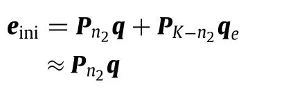
wherePn2=[p1,p2,...,pn2]is the firstn2principal components andPK−n2=[pn2+1,...,pK]is the remainingK−n2ones that explain little of the variance in data matrixX.q=[q1,q2,...,qn2]andqe=[qn2+1,...,qK]is the corresponding coefficients.

By estimating ˆq,the overall wind field could be approximated:

in which the termPn1is the estimated wind field from initial and boundary conditions,thePn2is the error compensation term based on the deviation of estimated wind field against sparse observations.The determination ofis given in Appendix A5.

2.6.Wind field reconstruction framework

A wind field reconstruction framework is finally prompted for specific congested environment.The ultimate goal is to retrieve stable wind field from both initial and boundary conditions and sparse observations.The overall reconstruction error is set as the proper criteria for the iteration to stop,given as:

The wind field reconstruction framework that integrates all the introduced algorithms is demonstrated in Fig.1.The initialization starts with the identification of meteorological parameter B for specific urban environment.Once the initial and boundary conditions are defined,CFD simulations are executed to generate database S.Proper sampling methods are used to generate the training data matrixXthat covers at least 70% of the scenarios.A full principal component decomposition is fulfilled on data matrixXto get principal componentsPand the corresponding coefficients matrixC.The truncation leveln0that the number of principal components that explain more than 99%of the variance in original data is calculated.In the mean time,the remaining scenarios are left for test purpose.A test scenario is randomly selected asbnew,xnew.

The iterative part starts by setting the number of principal componentsn2=n0to retrieve wind information from observations.Then,two streams are calculated in sequence.The right stream builds a regression model using ELM neural network.An inner iteration is designed to determine the bestn1for the residual of the regression model to reach its minimum.The left stream determinesn2≤m≤mmaxobservation locations by examining the step descent in the plot of WCEV (Eq.(5))vs.m.Then,the observation matrixHmis calculated.Given the ELM model,the preliminary estimated wind field ˆxiniis used to calculate the preliminary estimation error at selected observation spots.Finally,the error compensationeiniis added to the preliminary estimation to obtain the final results ˆxnew.The total reconstruction errorREis evaluated for the iteration to stop on specific conditions.

3.Numerical Case Study

3.1.Geometry configuration

This section introduces a numerical case study of 3D wind flow over obstructed area demonstrated in Fig.2.The domain inX,Y,Zdirections extends to 200 m,200 m and 50 m,respectively and theYaxis points to north.In the center of domain stands 9 cuboid buildings whose height ranges from 6 to 22 m.The size and location of these geometries are selected randomly.The rectangular obstacle other than ellipsoid and double sinusoidal model introduced in[22]will result in boundary layer separation at the edges.Horizontal vortices are generated in the wake areas.Besides,the narrow canyon between geometries produces Venturi effects that increase the wind speed.The main air flow will climb up in the windward side of geometry and downwash in the leeward to produce vertical vortices.

Fig.1.Wind field reconstruction and verification work flow.

3.2.Initial and boundary conditions

To simplify the scenario configurations,only averaged wind speed and direction at certain elevation are provided.The atmospheric stability is set to“D”.The remaining humidity,temperature and other meteorological parameters remain unchanged.The scenario parameter space B is generated by varying the wind speed(0.1-15 m·s−1)anddirection(0-360◦).Here,thewinddirectionisthedirectionwhere wind blows from,starting from north(0◦)and increasing clockwise.Fig.3 demonstrates 100 different scenarios created through HSS sampling method[26,27].Among these scenarios,90 are used to build the model and 10 are left for model validation.

Fig.2.Wind flow domain configuration.

Fig.3.Wind speed and direction configuration.(*):scenarios to build model;(◦):scenarios for validation.

3.3.CFD configuration

To launch the CFD simulation,the initial and boundary conditions should be initially defined.One important parameter is the vertical wind profile that follows the power law in simplicity:

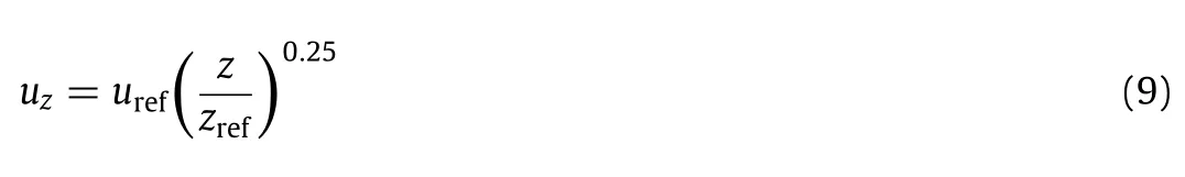
whereurefandzrefare the reference wind speed at reference elevation and the exponential value 0.25 is specified according to atmospheric stability“D”[28].Here,the reference height is set toZ=10 m.

Fig.4.Wind velocity sampling location in 2D(top view).

The fire dynamic simulator (FDS)[29]is selected as the CFD tool to calculate the wind flow over obstructed terrain.FDS is an open-source CFD package that has been used in smoke ventilation and gas dispersion simulations[30,31].FDS only supports structured cuboid mesh.The influence of grid size is evaluated on four settings:101 × 101 × 50,201 × 201 × 50,401 × 401 × 50 and 501 × 501 × 50.The values correspond to the number of grids inX,Y,Zaxis,respectively.The variations lies in the horizontal grid size,which is 2 m,1 m,0.5 m and 0.4 m.The corresponding number of grids is about 510k,2020k,8040k and 12550k,respectively(k stands for thousand).Since the goal of CFD simulation is to obtain detailed wind field data,9 spatial points on the height ofZ=5 m are selected(Fig.4)to record the wind velocity changes.Corresponding results are shown in Fig.5.Due to the turbulence in the wake of obstacles,there are no significant differences in the estimated wind velocity for each grid size.Finally,the mesh of 201 × 201 × 50 inX,Y,Zdirections is selected.The initial condition is defined as an initial wind field atZref.FDS provides a“nudging”technique to drive the computed wind field to the desired averaged wind speed,which is essentially a data assimilation process.The vertical wind profile is set through the built-in“RAMP”function.For the boundary conditions,the bottom face of the domain is set to“INERT”and all other faces are set to“OPEN”.The faces of obstacles inside simulation domain are also set to“INERT”.The desired simulation time for each scenario is 60 s,which is enough for the wind field to fully develop.

FDS implements Large Eddy Simulation(LES)for turbulence over grids and Smagorinsky subgrid-scale model for in-grid vortex.The detailed turbulence structures would be retained near the obstacles.Fig.6 demonstrates a sample wind field with the initial wind speed 10.11 m·s−1in 190.8◦.The dynamic behavior of the wind velocity field reaches a pseudo-steady state after about 30 s of simulation,corresponding to the requirements proposed in Section 2.1,which is the basis for the whole work flow to be feasible.

3.4.Hardware and platform

The FDS v6.5.3 package is launched on a workstation running openSUSE with dual-socket Intel® Xeon E5-2643 CPUs and 128 GB of memory.It takes about 45 h to simulate the 100 scenarios.The FDS code exports the wind velocity,wind component data across all mesh grids at each simulation second,which takes 238 GB of disk space in total.The wind field reconstruction model is developed in MATLAB R2017a,whose API is also utilized in a custom fortran code developed to covert the simulation results to MATLAB compatible data format.

Fig.5.Recorded wind velocity at spatial locations for different grid configurations.

4.Results and Discussion

To analyze the 2D wind field reconstruction,the horizontal layerZ=5 m is selected to make sure that all geometries could affect the wind flow.The simulation results contain wind velocity scalarUsand the wind componentsUx,Uy,UzinX,Y,Zdirection.The mesh of one horizontal layer is 201×201,containingN=40,401 features.Then,90 scenarios are randomly selected to generate the required data matrixX∈R40,401×90.From full principal component decomposition,89 independent principal components are extracted,explaining 100% of the variance inX.To launch the framework demonstrated in Fig.1,the truncation leveln0=7 is estimated on condition thatPn0retains at least 99%of the variance inX,as shown in Fig.7.The cumulative variance explained is plotted against the number of principal components.

The following subsections will elaborate the determination of the propern1the right stream andmin the left stream.The reconstructed wind field is evaluated against the original simulation results.

4.1.The regression model

The right stream aims at establishing the ELM-based regression model.TheELMalgorithmworksonasinglehidden-layerfeedforward neural network whose weight matrix and bias vector for the input layer are generated randomly.In the present paper,the number of neurons in the hidden layerLhis also fluctuating randomly between 20 and 120.

Fig.6.Snapshot of wind velocity field at Z=5 m at 40 s for scenario 94(topview).

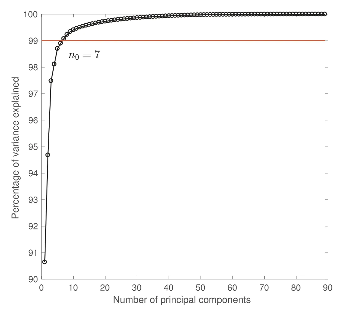
Fig.7.The cumulative variance explained by principal components.

During the model implementation,the condition number of the output matrixG(in Appendix A2.)reaches up to 1017,indicating that the linear problem is ill-posed.Thus,the general Tikhonov regularization is introduced by reforming the original problem to:

For a givenγ,the estimatedWis an optimal solution in the least square sense.WithW,the estimated coefficientis validated against the original coefficient matrix by calculating the following two Frobenius norms:

whereRsolis the norm of solution whileRresis the norm of residual.

The general way of determining the bestγis to generate an array of possibleγvalues and calculate the best estimation ofThe plotRresagainstRsolhas a corner(the point that has maximum curvature),corresponding to the bestγ[32],as demonstrated in Fig.8.

To determine the bestn1,the easiest way is to traverse all the possiblen1values and find the optimal one with minimum residual normRres(n1).The implementation of regression model is summarized in algorithm 1 in Appendix A2.

4.2.Sensing location

The left stream of the framework(Fig.1)acts as an error compensation to the estimated wind field from the right stream.Observations are integrated to improve the precision of reconstruction results.The selection of proper sensing location follows the MPME algorithms proposed in the literature[24],in which the criteria WCEV(Eq.(5))is used as a terminating threshold for the algorithm to stop.The MPME algorithm tries all the possible sensing locations to determine the best one at each iteration.The potential sensing locations are the grid nodes in the free space other than obstacles.If no more constraints are provided,the typical number of optional sensing locations would reach 37000.During the iteration,once a specific sensor location is determined,it will be excluded from the available location records for the next iteration.This raises a problem that the selected sensing locations might cluster in a limited area,which is prohibited in the real case.Thus,the Chebyshev distance is introduced to limit the minimal distance between two arbitrary sensing locations.In the 2D scenario,the Chebyshev distance of two locations(x1,y1)and(x2,y2)is given as:

By specifying appropriateD,once a sensing location is selected,the available optional locations withinDare all excluded for the next iteration.The following example demonstrates the effect of introducing Chebyshev distance in sensing location selection.The test scenario is also 94 withn2=20,DChe=10.The WCEV termination threshold is 1E5.

Fig.9 (a)shows three different sensing location configurations:the red“plus”is obtained withDChe=1 and the blue“circle”is obtained withDChe=10,the remaining green“diamond”is generated randomly.It is obvious that the selected sensors are clustered near the edges of obstacles 1,5,7 and 9 (red plus marker)with no additional constraints provided.In the configuration ofDChe=10,the selected sensors scatter near the edge of obstacles located at the outer region.The random sensor placement covers most of the free space evenly in domain.In Fig.9(b),the WCEV curve descends slower untilm=31 to reach the desired 1E5 threshold.On comparison,in Fig.9(c),the WCEV curve drops faster and requires only 29 sensors to reach the desired threshold.Due to the sensor clustering on condition ofDChe=1,it requires more iterations to jump out from the cluster to further decrease the average WCEV criteria.

4.3.Convergence settings

Once the sensor placement is set,the observation transition matrixHcould be calculated.The error compensation to the estimated wind fieldis then calculated based on sparse observation values.Finally,the overall wind field estimation could be achieved.The traditional way of stopping the iteration is to set specific threshold of reconstruction errorREand terminate the iteration once the calculatedREis smaller than the threshold.In this manuscript,it is difficult to determine the magnitude ofREassociated with different scenarios.A[NR]-validation check is designed for the algorithm to terminate.The algorithm keeps the latestNRreconstruction errorsREand calculates their variations.Generally,this variation is independent to scenario configurations and will decrease iteratively.Once the threshold ofNR-validation check is reached,the stable reconstruction result is obtained.

Fig.8.L-curve of coefficient matrix estimation for specific n1=24 and corresponding curvature.

4.4.Reconstruction results

From the dynamic visualization of the simulation results,it could be found that the wind field develops from idle state to the desired wind velocity and direction in about 30 s,then,the wind field reaches relative steady state.In this situation,the detailed streamlines in between the obstacles fluctuate in a small scale and the main trends remain unchanged.

To better meet the steady state requirement for the proposed reconstruction algorithm,a smooth filter is applied to the temporal varying data.The wind velocity and wind component values at specific timetare replaced by the averaged value within a time window containingLtime steps.The averaged data at 40 s with a smooth time window of 17 s are prepared for all the 100 scenarios.

Table 1 lists the key parameters of the reconstruction framework tested on scenario 94.Since either wind speed scalarUsor wind componentsUx,Uy,Uzare treated independently,the estimatedn2,n1andmare different.Besides,considering the difference in the values of the four physical fields,the stop criteria also varies to guarantee the convergence of the framework.It is obvious that the requiredn2,n1andmforUs,Ux,Uyare at the same magnitude,while those for the estimation ofUzare much larger.Here,n2andn1are the inner parameters that are not related to any real-world aspects.However,mindicates the number of required observation spots that should not be vary large.

Fig.10 (b,d,f,h)demonstrated the counter plot of estimated wind speed field and the corresponding wind component fields.By comparing with the original field in Fig.10 (a,c,e,g),the differences inUs,UxandUyare small that the high wind velocity region near the edge of obstacles is reproduced.However,theUzfield shows chaotic trends in reconstructed data that differs significantly from the originalUzfield,which is corresponding to the largest relative reconstruction error listed in Table 1.In the configuration of the 100 scenarios,vertical wind velocity is not defined.The value ofUzis calculated by solving the Navier-Stokes equation with interaction of obstacles.The downwash effect at the leeward side of obstacles induce a vertical spin,makingUzto change.From deep observation of Fig.10 (g),it could be found that there is an ascending wind front at the leeward edge of each obstacle (shown by the yellow line).Then the darker blue tails indicate the general descending wind flow further behind the obstacles.It is the result of a vertical vortex that appears near the top edge of the leeward side[33].Since the wind field reconstruction is executed on the 2D horizontal slice,the spatial features inUxandUyare well retained in data,however,the spatial features inUzare mostly contained in vertical slice data,not in the horizontal ones.The lack of features in data is the main cause of the poor reconstruction results ofUzshown in Fig.10 (h).Furthermore,since the data ofUzdo not contain enough features to describe its vertical vortex structures,they are more uncorrelated by takingn0=63 principal components to retain 99% of the variance,compared withn0=7 forUs(Fig.7).

For better comparison,the 2D vector field of reconstructed wind field and original wind field is demonstrated in Fig.11.The reconstructedwindfieldretainsthechannelflowcharacteristicsinbetween obstacles.Slight differences are noticed in the wake behind obstacles(bluevs.green arrows),however,the overall trends are well retained.

Table 2 gives the configuration of 10 test scenarios and the corresponding estimation results.The optimal model parameters and the overall estimation errorREare also included.As described in Section 2.2,the coefficient for the input layer of ELM neural network is generated randomly at each iteration,thus,the overall reconstruction errorREfor the same case might change during each estimation.This would explain the difference ofREfor scenario 94 in Tables 2 and 1.Among the 10 test scenarios,the maximum reconstruction error is found to be 13.08%,while the minimum is 5.56%.The averaged reconstruction error is around 9%.The 15-times repeated test indicates that the overall reconstruction errors fluctuate in small quantity around its average,as shown in Fig.12.One exception is the scenario 8,whose wind speed is the smallest among all the tested scenarios.The small wind speed might not be able to form a significant flow field that has obvious trend in between the obstacles.Despite the 9% of relative reconstruction error,the reconstructed wind fields coincide well with the original wind field and only a slight difference(similar to Fig.11)could be observed.

Fig.9.Demonstration of sensor location selection.(a)Three sensor placement configurations;(b)WCEV curve for DChe=1;(c)WCEV curve for DChe=10.

4.5.Practical strategy

The proposed framework provides a comprehensive schema in estimating the wind field.Initial conditions and local observationsare involved in determining the optimal parameters.However,in practice,most chemical plants are not equipped with enough meteorological sensors that cover the local facilities.The truth is that there would be roughly one major meteorological station within the 50-km range of the chemical plant,providing comprehensive observations on wind velocity,wind direction,humidity,temperature,pressure,solar radiation,etc.That means the left stream elaborated in Section 2.6 is usually unavailable.To distinguish different situations in reality,we denoted the default situation as situation (0)since both initial and boundary conditions along with sparse observations are provided.Then,the more realistic situation(1)is provided with relevant comprehensive weather monitoring information,while the local observations are unavailable.Situation(2)is provided with local observations,but the monitoring data from distant weather station is irrelevant.The operational usage of the proposed algorithm will be discussed in the two realistic situations.

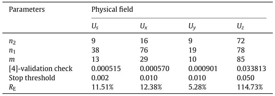
Table 1 Key reconstruction parameters of the algorithm for scenario 94

Fig.10.Original wind field compared with reconstructed results for scenario 94 at Z=5 m.(a,b)wind velocity Us;(c,d)wind component Ux;(e,f)wind component Uy;(g,h)wind component Uz.

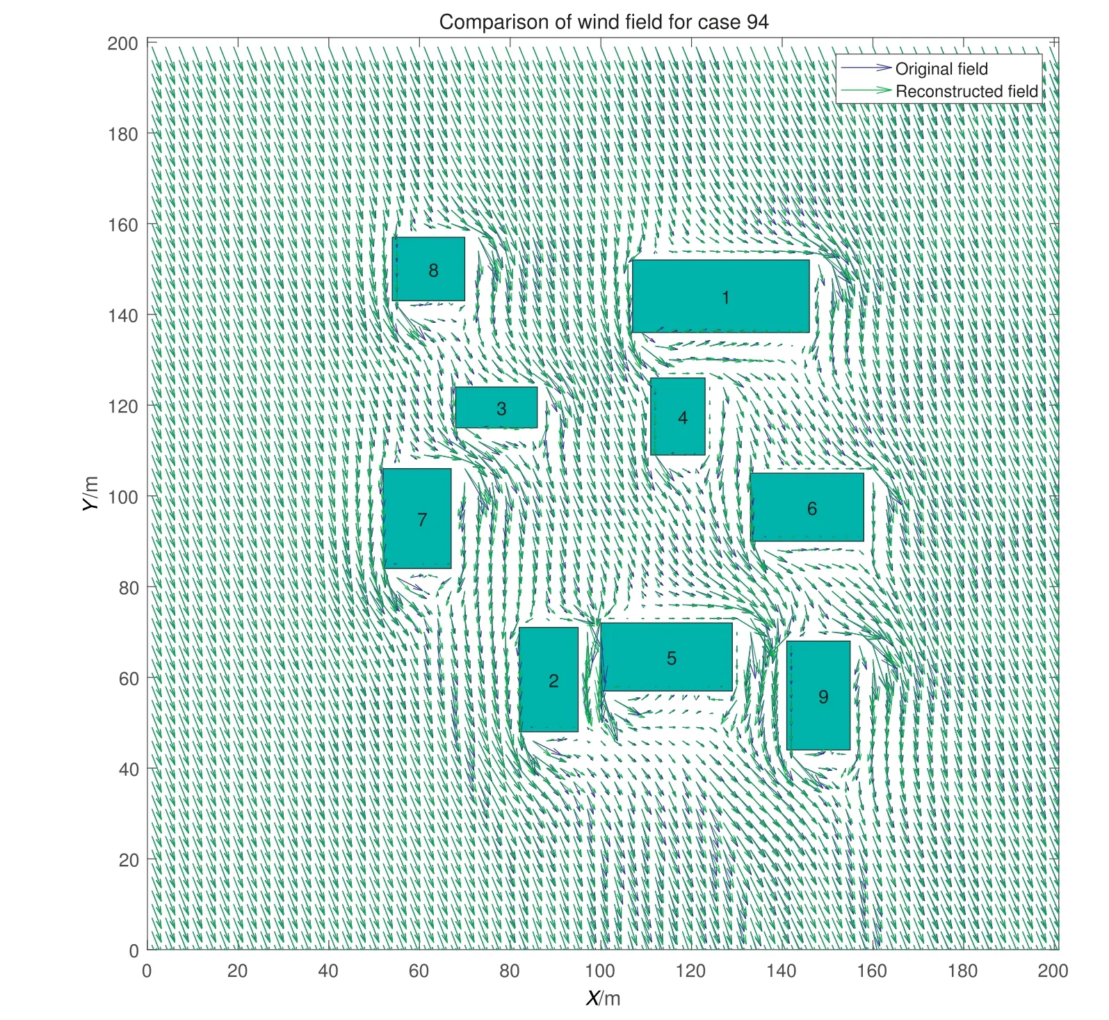
Fig.11.The comparison of reconstructed wind field and original wind field for scenario 94 at Z=5 m.

Situation(1)requires the left stream of the framework to be disabled since no error compensation is provided from local observation network.The reconstruction results depend on the initial and boundary conditions.In this situation,the reconstruction processes are more important for parameter tuning than the actual wind field estimation.To eliminate the stochastic parameterization embedded in the right stream,15 repeated trails are executed to find the optimal parameter configurations for highest accuracy.

Situation(2)assumes that only the local meteorological observations are available,meaning that the right stream is ignored.Then,the placement of meteorological sensors would be the key aspect on the accuracy of wind field reconstruction.The number of sensors is constrained by the number of principal componentsn2used to rebuild the wind field.In the framework,n2is determined by evaluating the performance improved at each iteration with the increase ofn2itself.However,it is impossible to determine the optimaln2in the operational stage because no“true”wind velocity data are available for the proposed framework to converge.

The significance of the proposed framework lies in exploring the dependency of model parameters on scenario configurations.Calm weather conditions with small wind velocity might require more sensors to track the chaotic details in wind field,while strong wind blast shows a significant flow trend and might save the number of sensors.The final choice of the parameter should also consider the frequency of scenarios based on historical observations.In the current manuscript,by assuming equal chance of the appearanceof 10 test scenarios,the framework is configured withn2=18,m=24 andn1=60.Then,the wind field reconstruction would be straight-forward since no iterations and convergence is needed.The adjustment of framework corresponds to the aforementioned situations.For situation (1),the framework is right-stream-only;for situation(2),framework is left-stream-only;for design situation(0),both streams are calculated.The averaged performances for each test scenario are presented in Table 3.The variation ofcorresponds to situation (1);corresponds to situation (2)andcorresponds to situation(0).In addition,the randomly scattered sensor placement is also tested for both situations (2)and (0)in the straight-forward manner.The results are denoted asand

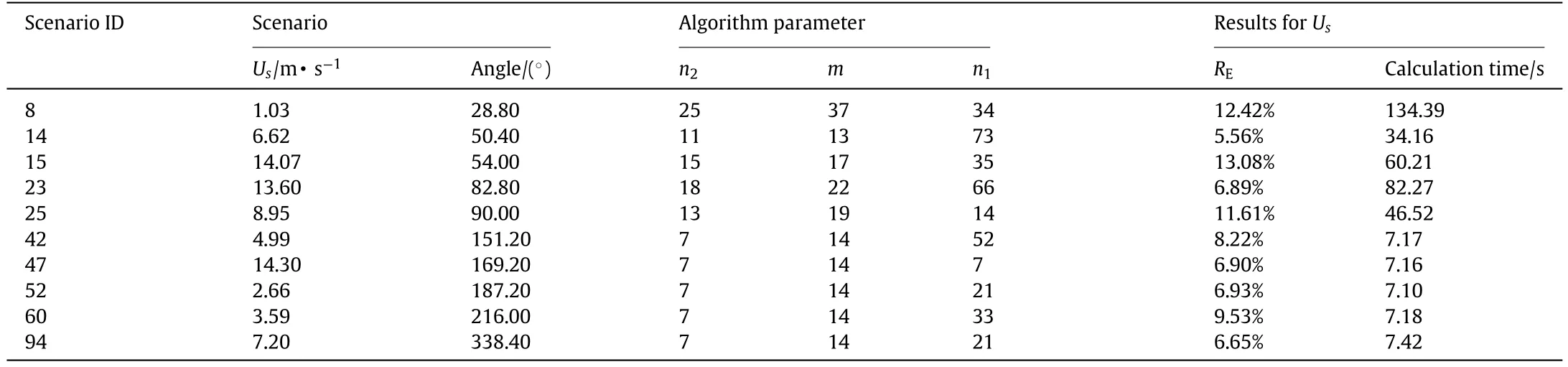
Table 2 Wind speed Us estimation parameters for 10 test scenarios at Z=5 m

Fig.12.The REof repeated test for all test scenarios.Legend shows the data markers corresponding to each test scenario.

The worst performance is found on scenario 8 with right-streamonly algorithm.The averaged reconstruction error reaches 685%.This reveals that for small wind scenario,the PCA-based model is not compatible to reproduce the wind field from single elevated observation.The linearity of the model might be lost.The same applies for scenario 52,which has the second smallest wind velocity among the test scenarios.Thebecomes smaller with wind velocityUsincreases.The performance improves for left-stream configurationssince additional information from local observation system is provided.Better results are obtained with combined-stream configuration

Table 3 Averaged reconstruction error in practical situation for 10 test scenarios on condition of n1=60,n2=18 and m=24

In the end,the proposed framework in Fig.1 provides a way of obtaining stable wind field reconstructions with minimum observation requirements.Unfortunately,it is impractical in real-world applications since no“true”wind field is known in prior.The proposed framework is more of an in-house verification method than a practical tool.But it actually provides adequate information in design stage to find the sub-optimal parameters(n1,n2andm)for operational wind field reconstruction.

5.Conclusions

The integrated wind field reconstruction framework for parameterization and verification has been proposed and successfully implemented in 2D urban environments.The framework takes information from both regional meteorological station and the local anemometer networks.The reconstruction model is built based on principal component decomposition,through which the high dimensional wind field data is reduced for better regression performance.The workable wind field reconstruction framework is implemented based on CFD data from 90 scenarios and verified on 10 independent test scenarios.

The proposed framework acts as a parameterization method since the optimal model parameters could be derived in the development process based on scenario specifications.Though the final convergence could not be achieved in the real-world situation,the scenario-optimal configurations of the sensor network and regression model would provide necessary information to set appropriate parameter value for operational use.The key parameters are the number of principal componentsn2used for error compensation and the corresponding sensor numbermon a balance of model accuracy and hardware costs.

Given abundant 3D CFD simulation results on wind flow over complex geometries,the framework could provide accurate wind field estimations with an averaged error of 9%for wind velocity scalarUsand the horizontal wind componentsUx,Uy.Since the reconstruction is implemented on horizontal 2D slice,the reconstruction ofUzis poor due to the lack of information on vertical turbulence,which is usually generated by rising air flow in the windward and downwash in the leeward.

In practical situation where convergence could not be guaranteed,the set of parameters,n1=60,n2=18 andm=24,are applied for thestraight-forwardwindvelocityreconstructionwitheitherabsence of initial conditions or local observations.The reconstruction errors for practical situations are acceptable around 12%.For low velocity scenarios reconstructed from initial and boundary conditions,the accuracy is poor because the linearity of PCA model might be lost.

In summary,the proposed framework provides an efficient way of reconstructing the wind field in a complex geometry along with the determination of optimal model parameters.The proposed work relies on the quasi-steady state assumption of wind field.No significant change should occur in wind direction and speed within the reconstruction time window.It should be mentioned that though the framework is implemented on horizontal 2D surface,the wind flow is simulated in 3D.In the manuscript,the data on horizontal sliceZ=5 m are used to build the framework.It is easy to extend the estimation of 2D wind field to any other height by simply taking the corresponding data and repeating the aforementioned procedures.Currently,the proposed 2D wind field reconstruction lacks the ability in estimating the vertical structure of wind flow,which might affect the vertical mixing of release substance and subsequently influence its ground level concentration distribution.Future work will emphasize on the extension to 3D wind field where vertical wind profile is considered.

Supplementary Material

Supplementary material to this article can be found online athttps://doi.org/10.1016/j.cjche.2019.02.029.