Yingjun Wang , Zhen p ei Wang , Zhaohui Xia and Leong Hien Poh

Abstract: Isogeometric analysis (IGA), an approach that integrates CAE into conventional CAD design tools, has been used in structural optimization for 10 years, with plenty of excellent research results. This paper provides a comprehensive review on isogeometric shape and topology optimization, with a brief coverage of size optimization. For isogeometric shape optimization, attention is focused on the parametrization methods, mesh updating schemes and shape sensitivity analyses. Some interesting observations, e.g. the popularity of using direct (differential) method for shape sensitivity analysis and the possibility of developing a large scale, seamlessly integrated analysis-design platform, are discussed in the framework of isogeometric shape optimization. For isogeometric topology optimization(ITO), we discuss different types of ITOs, e.g. ITO using SIMP (Solid Isotropic Material with Penalization) method, ITO using level set method, ITO using moving morphable com-ponents (MMC), ITO with phase field model, etc., their technical details and applications such as the spline filter, multi-resolution approach, multi-material problems and stress con-strained problems. In addition to the review in the last 10 years, the current developmental trend of isogeometric structural optimization is discussed.

Keywords: Isogeometric analysis, structural optimization, shape optimization, topology optimization, sensitivity analysis.

1 Introduction

Structural optimization, as an important tool in the product design process, deals with the optimal design of load-carrying structures. In general, structural optimization methods can be divided into three categories: S ize, shape and topology optimization methods [Bendsoe and Sigmund (2003); Huang and Xie (2010); Mortazavi and To˘gan (2016); Tejani, Savsani,Patel et al. (2018)]. An illustration of these three types of structural optimization is shown in Fig. 1. Size optimization deals with the optimum size parameters such as cross-section dimensions and thickness, while fixing the shape and topology of the structure. Shape optimization works by modifying the outer boundary of the structure to obtain the optimal shape. Topology optimization optimizes the material layout within a given design domain,which is capable to find the o ptimal t opology from d i fferent topologies rather t han a particular topology. Of the three categories, size optimization is a relatively simple parameter optimization. We will thus focus on the other two types of structural optimization in this review.

In shape optimization, the geometric parameterization, an adequate boundary description and the design variables are essential for a successful optimization. To be consistent with the analysis model, the coordinates of the boundary nodes were used as design variables in the early days of shape optimization [Francavilla, Ramakrishnan and Zienkiewicz (1975)].However, utilizing the nodal coordinates as design variables may result in unrealistic designs with irregular boundaries [Haftka and Grandhi (1986); Hsu (1994)]. To avoid such irregular optimized results, researchers tried to use geometric boundary representations in shape optimization, such as polynomials, B-spline and NURBS [Ding (1986); Samareh(2001a)]. Although the usage of spline representations improves the smoothness of boundaries, the design model based on splines is separated from the analysis model based on finite element, resulting in a disconnection between the design and analysis models. To update the shape geometry during the iterative process of shape optimization, a relation between the design variables and the analysis model is required, e.g. the design element [Imam(1982)] and the natural design variables [Belegundu and Rajan (1988)]. Besides, some strategies such as adaptive meshing [Bennett and Botkin (1985)] and remeshing [Wilke,Kok and Groenwold (2006)] are required to maintain the accuracy of shape optimization,especially for the shape optimization with large deformations.

Figure 1: An illustration of structural optimization

Shape optimization cannot change the topology of the structure so it is usually used to optimize the detailed features of the product after the basis geometrical shape has been obtained. In contrast, topology optimization aims to find the optimal material distribution in a design domain, such that the structural topologies can change during the optimization process. The first attempt was made by Cheng et al. [Cheng and Olhoff (1981)] on optimal thickness distribution of solid elastic plates, and the pioneering work of Bendsøe and Kikuchi [Bendsøe and Kikuchi (1988)] that used a homogenization method to generate the optimal topologies was a milestone in the topology optimization research. Since then,other important methods have been proposed to solve topology optimization problems, e.g.solid isotropic material with penalization (SIMP) [Bendsøe (1989); Sigmund (2001); Andreassen, Clausen, Schevenels et al. (2011)], evolutionary structural optimization [Xie and Steven (1993); Querin, Steven and Xie (1998); Huang and Xie (2009)] and level-set based topology optimization [Wang, Wang and Guo (2003); Allaire, Jouve and Toader (2004);Luo, Tong, Wang et al. (2007); Xia, Shi and Xia (2019)]. Topology optimization is becoming an efficient tool in product designs, and has been applied to a wide range of engineering domains such as aerospace [Zhu, Zhang and Xia (2016)], automobile [Yang and Chahande(1995)], additive manufacturing [Mass and Amir (2017)] and photonics [Borel, Harpøth,Frandsen et al. (2004)].

The abovementioned shape and topology optimization methods are based on the finite element method (FEM), some limitations of the FE approach include the disconnection between analysis and geometric models, low continuity between the elements and low efficiency of high-order elements. These limitations are successfully addressed by a new method called isogeometric analysis (IGA) [Hughes, Cottrell and Bazilevs (2005)], which directly uses the basis functions of a computer aided design (CAD) model as the shape functions of analysis model, IGA has since been used in a variety of domains [Benson,Bazilevs, Hsu et al. (2011); Hsu and Bazilevs (2012); Wang and Benson (2015); Wang,Benson and Nagy (2015); Yan, Deng, Korobenko et al. (2017); Deng, Wu, Yang et al.(2018)]. In the last decade, IGA has been adopted for both shape and topology optimizations, which provides several advantages over the established methods. For example, the exact geometric representation of IGA merges analysis and design model in shape and topology optimizations [Wall, Frenzel and Cyron (2008); Seo, Kim and Youn (2010b,a)],and the spline functions of IGA can avoid the checkerboards in the topology optimization without additional filters [Hassani, Khanzadi and Tavakkoli (2012); Dedè, Borden and Hughes (2012); Lieu and Lee (2017a)]. Although the research in isogeometric structural optimization has been growing for the past decade (See Fig. 2), to the best of our knowledge, no comprehensive review has been published yet to help the researchers working in this domain to systematically understand isogeometric structural optimization.

In this paper, we intend to provide a comprehensive review on the isogeomtric structural optimization from the first work of Wall et al. [Wall, Frenzel and Cyron (2008)] proposed in 2008. An outline of the remainder of this paper is as follows: Section 2 introduces the fundamentals of isogeometric structural optimization. Section 3 gives a comprehensive review for isogeometric shape optimization including shape sensitivity analysis, regulation method, special application etc. Section 4 discusses different types of isogeometric topology optimization (ITO) including but not limited to density-based and level-setbased ITOs. The conclusions and research trends are provided in Section 5.

Figure 2: Numbers of publications on IGA and isogeometric design optimization per year(data from Scopus search engine)

2 Fundamntals of isogeometric structural optimization

Isogeometric analysis (IGA), proposed by Hughes et al. [Hughes, Cottrell and Bazilevs(2005)], is an efficient alternative to conventional FEM, which represents the analysis model with CAD mathematical primitives such as B-spline and NURBS. Over ten years of development, IGA is now the most active research topic in both computational mechanics and computer aided geometric design, and has been applied to solve many problems in-cluding structural optimizations. In this section, we will summarize the fundamentals of isogeometric structural optimization consisting of IGA and structural optimization.

2.1 Summary of isogeometric analysis

2.1.1 Numerical geometry description tools

A number of new spline technologies have been used in IGA, including T-splines [Bazilevs,Calo, Cottrell et al. (2010); Scott, Li, Sederberg et al. (2012)], PHT-splines [Nguyen-Thanh,Kiendl, Nguyen-Xuan et al. (2011)] hierarchical B-splines or NURBS [Vuong, Giannelli, Jüttler et al. (2011); Wu, Huang, Liu et al. (2015)] and Powell-Sabin splines [Speleer-s, Manni, Pelosi et al. (2012)]. Presently B-splines and nonuniform rational B-splines (NURBS) [Piegl and Tiller(1997)] are commonly used in CAD systems, and are still the most prevalent spline technology in IGA. In B-splines, the a knot vector Ξ = {ξ1, ξ2, ..., ξn+p+1} is a sequence of non-decreasing real numbers in the parametric space, where n is the num-ber of control points and p is the order of the spline curve. The interval [ξ1, ξn+p+1) is called a patch and the knot interval[ξi, ξi+1) is called a span. The B-spline basis functions can be recursively defined by the Cox-de Boor formula [Boor (1972)]:

The continuity of the B-spline basis functions between knot spans is Cp-kwith k as the multiplicity of the knots.NURBSbasis functions can be defined based on B-spline basis function by assigning apositiveweight wito each basisfunction or control variables:

Notethat B-splinesareaspecial caseof NURBSwheretheweightsareuniform.A pointlocation vector x(χ)in ageometry patch described using NURBScan begenerally expressed as

whereχisthelocation vector in theparametric space:

I is a index function with a form of I(i)for 1D problems,I(i,j)for 2D problems and I(i,j,k)for 3D problems;the weighted basis function RIis obtained from the tensor products of the 1D case shown in Eq.(2)along different directions and correspond to the I th control point xI.

Taking two dimensional B-splinefor example,thebasisfunctionsareconstructed astensor products,

Bi,p(ξ)and Bj,q(η)areunivariate B-spline basisfunctionsof order p and q,corresponding to knot vectors Ξ ={ξ1,ξ2,...,ξn+p+1}and H={η1,η2,...,ηm+q+1}.According to thetensor product formulation,two-dimensional NURBSbasis functionswith order p inξ direction and order q inηdirection areconstructed as

Thefour important propertiesof NURBSbasisfunctions(likewise for B-spines)arebriefl y listed as:(1)Nonnegativity:Ni,j(ξ,η)≥ 0;(2)Partitionof unity1;(3)Local support:Ni,j(ξ,η)=0 if(ξ,η)is outside the span domain of[ξi,ξi+p+1)×[ηj,ηj+q+1);and(4)Continuity:the interior of knot span domain iscontinuousup to C∞,and the continuity between knot spansare Cp-kand Cq-lwhere k and l are the multiplicity,respectively.

2.1.2 NURBS-based IGAfor solving boundary valueproblems

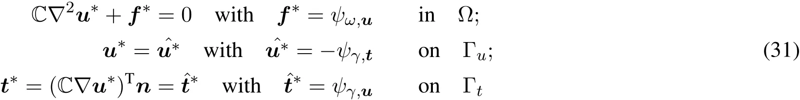
A typical boundary value problem formulation defi ned over domainΩwith boundaryΓ can beinterpreted as

where c(u)represents theequilibrium equation,f is body force,C is a forth-order tensor related tomaterial properties,n istheoutward normal vector,div isthedivergenceoperator,∇is the gradient operator,ˆt andˆu are the prescribed Neumann and Dirichlet boundary conditionsdefined onΓtandΓu,respectively.

Introducing a test function fi eld¯u,the weak formulation of the strong form defi ned in Eq.(6)can be written as:

This BVPcan besolved using fi niteelement method.Using the Bubnov-Galerkin method,thestatevariable u and theforcefi eld arediscretized and subsequently substituted into Eq.(7)to obtain a system of linear equationssuch that the problem can be solved:

where K is the stiffness matrix,U is the unknown discrete variables and F is a force vector.Note that the terminology used here originated in mechanical problems for the development of FEM and can beused to non-mechanical problemsthat may havedifferent terminologies.

The NURBS-based IGA follows a similar approach to obtain Eq.(8),but the shape functionsused for discretization arethesameasthebasisfunctionsused for geometry description,i.e.the the state variablesand theforcefi eld are discretized using the basis functions in Eq.(3).In theframework of IGA,thestatevariable u isinterpolated as

where uIis the state variable vector of the I th control point xI.Using this interpolation scheme,theelement stiffness matrix Kethat can bewritten as

Table1:Comparison Between IGA and FEM

where B represents thestrain-displacement matrix,D denotes thestress-strain matrix,Ωerepresentstheelement domain,isthemapping domain in the NURBSparametric space,andis integration domain in the integration parametric space.Jacobian J1and J2indicate the transformation relation from the NURBSparametric space to the physical space and the integration parametric space to the NURBSparametric space,respectively.Moredetailscan befound in Wang et al.[Wang,Xu and Pasini(2017)].

Compared with conventional FEM,IGA has a series of advantages such as nonnegativity and high continuity for high-order basis functions.A comparison between IGA and FEM is shown in Tab.1.It is noted that the geometry remains constant when elements are refi ned in IGA,since IGA uses the accurate geometric model.This is not true with FEM,which uses finite elements to approximately discretize the geometric models.Besides,the accuracy per degree of freedom(DOF)can be improved by the smoothness of splines in IGA.

2.2 Basisstatement of structural optimization

A typical structural optimizationprobleminvolvesasetof designvariables d=(d1,d2,···),an objective functionΨ?u(x);d?,a system of equality constraints charactered by the boundary value problem(BVP)defined in Eq.(6),and some other constraints,which can beexpressed as:

where the constraint defi ned by the BVPis nested in a weak form〈c(u),¯u〉Ω=0;x is location vector;hiare equality constraints;and giare theinequality constraints.

The above formulation of a structural optimization problem is based on continuum variables.An alternativeinterpretation isto defi netheproblem based on discreteformulations:

where the variables have been discretized.

In general, the gradient of the objective and constraint with respect to the design variables needs to be calculated so that a gradient-based method such as steepest descent method[Boyd and Vandenberghe (2009)], sequential quadratic programming (SQP) [Boggs and Tolle (1995)], the optimality criteria (OC) method [Hassani and Hinton (1998)], convex linearization method (CONLIN) [Fleury (1989)], the method of moving asymptotes (MMA) [Svanberg (1987)] and Globally convergent version of MMA (GCMMA) [Svanberg(2002)] can be used to solve the optimization problem. There are also non-gradient-based methods such as genetic algorithm (GA) [Adeli and Kumar (1995)] and Particle swarm optimization (PSO) [Eberhart and Kennedy (1995)] to solve the optimization problem with absence of the gradient, but the efficiency of such non-gradient-based methods is much lower compared to the gradient method.

3 Isogeometric shape optimization

Structural shape optimization is a type of design methodology that optimizes structures by changing the geometry shape such that a cost function is minimized. It has been a research interest since 1970s [Haftka and Grandhi (1986)]. As the computational mechanics was restricted by the computational resources at that time, the effectiveness of the size and topology optimization was limited. Meanwhile, shape optimization was able to provide optimal designs suitable for practical applications. Hence it was considered as a more effective design method. However, compared to size and topology optimization where the finite element mesh remains same and the perturbations of the design variables only affect the material property tensor, shape optimization is relatively more challenging because (i) it often requires the finite element mesh to be updated during an iterative optimization process and (ii) the perturbation of the design variables directly affects the geometry boundary and the integration domain. This poses three critical problems: the parameterization method,shape updating scheme and the sensitivity analysis.

With IGA, a seamless integration between analysis and design is achieved, and hence automatically averts typical parameterization problems in traditional FEM-based shape optimizations. Compared to FEM-based shape optimizations, there are three additional advantages of isogeometric shape optimization [Wall, Frenzel and Cyron (2008); Cho and Ha (2009)]: (i) its ability of preserving the curved geometry features for analysis, which makes it ideal to design structures or domains with curved boundary features; (ii) its higher accuracy of evaluating structural responses, especially for boundary variables and dynamic responses, which is desirable for sensitivity analysis involving boundaries and interfaces;and (iii) the integrated design-analysis-optimization model, which can significantly reduce the transition effort between CAD and analysis models. With these two advantages, isogeometric shape optimization method has demonstrated its capability in designing curved domains, e.g. Nagy et al. [Nagy, Abdalla and Gürdal (2010a); Hosseini, Moetakef-Imani,Hadidi-Moud et al. (2018); Choi and Cho (2018a); Weeger, Narayanan and Dunn (2018);Liu, Yang, Wang et al. (2018)] about curved beams; Nagy et al. [Nagy, IJsselmuiden and Abdalla (2013); Kiendl, Schmidt, WWüchner et al. (2014); Kang and Youn (2016); Bandara and Cirak (2018); Hirschler, Bouclier, Duval et al. (2018)] about shells; Gillebaart et al. [Gillebaart and De Breuker (2016); Herath, Natarajan, Prusty et al. (2015); Kostas,Ginnis, Politis et al. (2015, 2017)] about fluid-interacted structural geometries; Nagy et al.[Nagy, Abdalla and Gürdal (2011); Manh, Evgrafov, Gersborg et al. (2011); Taheri and Hassani (2014)] about dynamic problems; Wang et al. [Wang, Poh, Dirrenberger et al.(2017); Wang and Poh (2018); Choi and Cho (2018a)] about smoothed curved auxetics; Hao et al. [Hao, Wang, Ma et al. (2018)] with reliability-based design optimization;and Nguyen et al. [Nguyen, Evgrafov and Gravesen (2012); Pels, Bontinck, Corno et al.(2015)] about magnetic-related design domains. The integrated analysis-design framework enables to build a platform where the structural responses of designs with different parameters can be observed easily, and hence a sequence of the results can be used as samples for a surrogate model to quickly explore the design space [Benzaken, Herrema, Hsu et al.(2017)].

In this section, the issues of parameterization methods, shape updating schemes and sensitivity analysis in the context of isogeometric shape optimization is comprehensively reviewed with comparisons to traditional-FEM based shape optimizations in Sections 3.1 and 3.2. Studies based on gradient-free optimization methods are discussed in Section 3.3. Some remarks and discussions about isogeometric shape optimization are briefly summarized in Section 3.4.

3.1 Design parameterization, analysis techniques and updating schemes

3.1.1 Parameterization methods in traditional FEM-based shape optimization

A major limitation with the traditional FEM-based shape optimization lies with the transition between a geometry model described in a CAD system and the analysis model discretized with finite element mesh. Depending on the design parametrizations, different approaches have been developed.

An intuitive way is to use the finite element mesh directly, with the nodal locations as design variables (e.g. [Zienkiewicz (1973)]). This is also termed as a "parameter-free"approach (e.g. [Le, Bruns and Tortorelli (2011); Riehl, Friederich, Scherer et al. (2014)] ).This approach naturally avoids a CAD description and hence the corresponding transition difficulties. However, in addition to introduce a large number of design variables, it also leads to non-optimal jagged boundaries and irregular meshes, as illustrated in Fig. 3,and the geometry features such as curvature can only be approximated [Schmitt and Steinmann (2017)].

Figure 3: Schematic of jagged boundaries occurring during a shape optimization for a FEM-based shape optimization

An alternative approach is to use parametric curves or surfaces to describe the design objects. These parametric schemes include polynomials (e.g. [Imam (1982)]), Bezier and BSplines (e.g. [Braibant and Fleury (1984, 1985)]), NURBS (e.g. [Schramm and Pilkey(1993)]), mesh mapping/morphing (e.g. [Wang, Zhang, Wang et al. (2010); Wang, Wang,Zhu et al. (2011)]) and bi-space parametrization (e.g. [Wang and Zhang (2012); Wang,Zhang and Zhu (2016)]). More details of the parameterization can be found in the surveys of Haftka et al. [Haftka and Grandhi (1986); Samareh (2001b); Daxini and Prajapati(2017)]. The two major advantages of using a parametric method for shape optimization lie in two major aspects: (i) to reduce the number of design variables; (ii) to improve the accuracy of shape sensitivity analysis. However, the disadvantage of using a separate description for the geometry is that the mesh updating process requires the transition between parametric and analysis models. One tricky way of avoiding the mesh updating problem is to embed the structural domain on a background mesh where only the domain covered regions are assumed to have solid material, with the remaining domain composing of voids(e.g. [Bendsøe (1989); Norato, Haber, Tortorelli et al. (2004); Wang and Zhang (2013)]).Generally, the level-set-based topology optimization is a variant of this method, which will be addressed later in section Section 4.2.

3.1.2 Isogeometric shape optimization with different parameterization methods and analysis techniques

Figure 4: Double levels of discretization scheme: (a) A coarse discretization for design parameterization to reduce design variables and (b) A refined discretization for analysis to guarantee accurate structural responses [Wang, Turteltaub and Abdalla (2017); Wang,Abdalla and Turteltaub (2017)]. Note that an interesting observation is found in Lieu et al.[Lieu and Lee (2017a,b)] for isogeometric topology optimization, an contrary strategy is used such that a coarse mesh is used for analysis to improve the computational efficiency,yet a refined mesh is used for design to achieve topology designs with a high resolution

In the framework of isogeometric analysis, the transition between geometry description and analysis model is seamless. Hence, using IGA for shape optimization automatically avoids the problems induced by the parameterization approaches, and naturally leads to a simple integrated design framework. This was first addressed in the pioneering works [Wall, Frenzel and Cyron (2008); Cho and Ha (2009)]. Since the NURBS refinement can be easily achieved using standard algorithms to insert knots into the knot vectors, the isogeometric shape optimization framework also provides a platform to use multilevels discretization for design and analysis [Nagy, Abdalla and Gürdal (2010a)],e.g. a coarse discretization for design variables to reduce the number of design variables and a refined discretization for analysis to ensure the accuracy, as illustrated in Fig. 4. It should be noted that in [Lieu and Lee (2017a,b)] for isogeometric topology optimization, an contrary strategy is used such that a coarse mesh is used for analysis to improve the computational efficiency, yet a refined mesh is used for design to achieve topology designs with a high resolution. Although NURBS is a powerful tool to describe complicated geometries, the CAD models are not always analysis-suitable [Schmidt,Kiendl, Bletzinger et al. (2010); Scott, Li, Seder-berg et al. (2012); da Veiga, Buffa,Cho et al. (2012)], especially for complex geometries such as structures with cut-out openings using Boolean operations. This strongly restricts the development of isogeometric shape optimization. This problem can be solved using two approaches: one is to propose new parameterization methods that are analysis-suitable; the other one is to develop new analysis techniques to conform to existing CAD modeling methods.For such purposes, various parameterization methods and analysis techniques have been developed to further promote the design optimization. Representative parameterization methods include analysis suitable T-splines in Scott et al. [Scott, Li, Sederberg et al.(2012); da Veiga, Buffa, Cho et al. (2012)], an analysis-suitable parameterization framework using harmonic method in Xu et al. [Xu, Mourrain, Duvigneau et al.(2013)], a method of using mapped B-spline basis functions in [Yuan and Ma (2014)]and an optimized trivariate B-spline solids parameterization approach in Wang et al.[Wang and Qian (2014)]. Representative analysis techniques for shape design optimization problems in-clude the T-Spline based IGA in Ha et al. [Ha, Choi and Cho (2010)], boundary element method (BEM) based IGA in Li et al. [Li and Qian(2011); Lian, Kerfriden and Bordas (2016); Yoon and Cho (2016)], a combination of TSpline and BEM solver in Schillinger et al. [Schillinger, Dede, Scott et al. (2012);Kostas, Ginnis, Politis et al. (2015); Yoon, Choi and Cho (2015); Lian, Kerfriden and Bordas (2017); Kostas, Fyrillas, Politis et al. (2018)], Powell-Sabin splines based IGA in Speleers et al. [Speleers and Manni (2015)], isogeometric B-Rep analysis for trimmed surfaces in Philipp et al. [Philipp, Breitenberger, D’Auria et al. (2016)], an immersed method termed immersogeometric methods in Wu et al. [Wu, Kamensky, Wang et al.(2017)], an combination of immersed method and bound-ary method in Marco et al.[Marco, Ródenas, Fuenmayor et al. (2018)], and triangulations based IGA in Wang et al.[Wang, Xia, Wang et al. (2018)]. It should be noted that among these methods, the boundary element method is popular for its certain advantages over the domain-based methods, e.g. the unnecessary of generate domain mesh such that the interior mesh irregularity can be avoided during an optimization process. With the development of IGA,analysis-suitable parameterization techniques can provide a truly seamless analysisdesign environment that is capable of dealing with complex geometries for multi-physics problems, e.g. the works in Herrema et al. [Herrema, Wiese, Darling et al. (2017)].

3.1.3 Shape and mesh updating schemes

For the traditional FEM-based shape optimization, it is important to use proper mesh updating techniques to deal with the jagged boundary and irregular mesh. These techniques include the traction method that takes the shape derivatives on the boundary as a type of Neumann boundary condition in Inzarulfaisham et al. [Inzarulfaisham and Azegami (2004);Azegami and Takeuchi (2006); Shimoda, Tsuji and Azegami (2007); Riehl, Friederich,Scherer et al. (2014)], an automatic regridding method that takes the shape derivatives on the boundary as a type of Dirichlet boundary condition in Choi et al. [Choi and Kim(2005a)] and filtering method in Bletzinger et al. [Bletzinger, Firl, Linhard et al. (2010);Le, Bruns and Tortorelli (2011); Firl, Wüchner and Bletzinger (2013)].

In the framework of isogeometric shape optimization, although it is mentioned in Braibant et al. [Braibant and Fleury (1984, 1985)] that a B-Spline parameterization automatically accounts for boundary irregularities, proper boundary and domain mesh regularizations are still required. This mainly because that (i) the boundary shape change may cause irregular mesh if the interior control points are not moved properly [Yuan and Ma (2015); Choi and Cho (2015)] and (ii) the non-uniform local supports of the control points can lead to unbalanced step-sizes for different design control points to give an irregular geometry [Nagy(2011); Wang, Abdalla and Turteltaub (2017)], as illustrated in Fig. 5. To address these problems, several methods have been developed. For simple problems, it is possible to use a linear interpolation scheme for relocating the interior control points, e.g. the works in Wang et al. [Wang, Abdalla and Turteltaub (2017)]. In Nagy et al. [Nagy, Abdalla and Gürdal (2010a)], a Sobolev semi-norm, referred to as "shape change norm", is proposed. In Azegami et al. [Azegami, Fukumoto and Aoyama (2013)], the H1 gradient method, which is essentially similar to the traction method, is utilized. Both the shape change norm and the H1 gradient methods require to solve a system of equations. In Yuan et al. [Yuan and Ma (2015)], a parametric mesh regularization based on a method of mapped basis functions is demonstrated with a iterative procedure. In Choi et al. [Choi and Cho (2015)], a mesh regularization scheme is proposed by minimizing the Dirichlet energy functional and a dimensionless functional such that the uniform parametrization and the mesh orthogonality can be obtained. In Kiendl et al. [Kiendl, Schmidt, WWüchner et al. (2014)], a sensitivity weighting method is presented to normalize the step-sizes of the movements of the control points. This approach is further studied systemically in Wang et al. [Wang, Abdalla and Turteltaub (2017)], where additional normalization approaches are proposed and the underlying reasons of using the normalization approaches analysed.

3.2 Shape sensitivity analysis methods

Shape sensitivity analysis plays a critical rule in a gradient-based optimization process. In this work, we distinguish between the various sensitivity analysis methods based on how the derivatives of the state variable field are treated, to give t he: (i) Direct method (DM);(ii)Overall finite d ifferences ( OFD); ( iii) S emi-analytical ( SA) m ethod; a nd ( iv) adjoint method. An alternative classification method used in the surveys of [Van Keulen, Haftka and Kim (2005); Newman III, Taylor III, Barnwell et al. (1999)] is based on whether the derivation is derived from a continuum or discrete forms. This classification is also used here to have a comprehensive discussion for each type of sensitivity analysis method, e.g. for the adjoint method, it is further distinguished into two types: (i) Discrete adjoint method and (ii)Continuum adjoint method, also known as continuous or variational adjoint method (see e.g.[Newman III, Taylor III, Barnwell et al. (1999); Choi and Kim (2005a,b)]). The fundamental aspects of these sensitivity methods were developed in the 1980s, and become increasingly applicable for shape optimization problems with the development of software and hardware platforms for numerical analysis. Since surveys and reviews have been avail-able for these informations in the works of Adelman et al. [Adelman and Haftka (1986); Haftka and Adelman (1989); Tortorelli and Michaleris (1994); Hsu (1994); Newman III, Taylor III,Barnwell et al. (1999); Van Keulen, Haftka and Kim (2005)], we will focus on shape sensitivity analyses in the context of isogeometric shape optimization.

3.2.1 Preliminaries: M aterial derivatives and transport relations

For simplicity, the problem here assumes that the load is design-independent. Henceforth,to elaborate on the shape sensitivity analysis methods for the continuum-based formulations shown in Eq. (11), we defi ne the objective function in a generic manner as

where s isatime-likeparameter,analogousto thetimeparameter in continuum mechanics.In analogy to the configuration change with time in continuum mechanics,the material derivative,also termed material design derivative in Wang et al.[Wang and Turteltaub(2015)]to distinguish with the material time derivatives(e.g.in Jao et al.[Jao and Arora(1992);Wang and Kumar(2017)])of time-dependent problems,of a generic function f(x;s)isdefi ned as where(·)= (˙·)denotes the material or total derivatives of a quantity,=f′is the spatial(design)or partial derivativesandνisthedesign velocity fi eld:

Figure 5:The design parameterization dependency of NURBS-based shape updating scheme[Wang,Abdalla and Turteltaub(2017)]:Case 1 corresponds to a parameterization with uniformly distributed control points,uniform weights w|y=0,5,10 ={1,1,1,1,1,1}and uniform knot spansξ={0 0 0 0.25 0.5 0.75 1 1 1};Case 2 corresponds to a parameterization with uniformly distributed control points,uniform weights w|y=0,5,10={1,1,1,1,1,1}and non-uniform knot spansξ={0 0 0 0.1 0.2 0.3 1 1 1};Case 3 corresponds to a parameterization with uniformly distributed control points,non-uniform weights w|y=0 = {1,1,0.6,0.6,1,1}and uniform knot spansξ ={0 0 0 0.25 0.5 0.75 1 1 1};Case4 correspondsto aparameterization with non-uniformly distributed control points,uniform weights w|y=0,5,10={1,1,1,1,1,1}and uniform knot spansξ={0 0 0 0.25 0.5 0.75 1 1 1};Case 5 corresponds to a parameterization with linear basisfunctionsand non-uniformly distributed control points

The symbol V in Eq.(15)denotes the perturbation of point x with respect to design variable di.Note that in many references,e.g.[Cho and Ha(2009)],for simplicity,the definition of thetime-likeparameter isabsence,and thequantity V defined hereisused as‘design velocity’.Essentially,thereisno differencebetween thesetwo terminologies.

Thetransport relationsfor domain and boundary integralsareexpressed,respectively,as

and

whereκisthe mean curvature and n isthe unit outward normal vector.

3.2.2 Direct method

The direct method(DM),also called direct differentiation method(e.g.[Arora(1993);Tortorelli and Michaleris(1994);Cho and Ha(2009)]),is to take the derivatives of the objective functionΨwith respect to the design variables diusing the chain rule.For both continuum and discrete approaches,the DM requires to solve the system of equations in Eq.(8)to obtain thediscrete state variable field U,such that thecontinuum state variable u can beevaluated at any given location.

Using thetransport relation defi ned in Eqs.(16)and(17),thecontinuum-based derivatives of the objective function reads

whereνn= ν ·n.Then,thetransport relationsareapplied to theweak formulation in Eq.(7)to obtain itsderivatives.Notethat thespatial derivativesof thetest function¯u vanishes using〈c(u),=0.Following this,discretization isapplied to obtain adiscretesystem:

where U′is the vector of the spatial derivative of the discrete state variables and T is a dummy forcevector that is afunction of u,∇u,κ,n and V.Eventually,solving Eq.(19)and usetheresult to obtain u′in Eq.(18),theshapesensitivity can beevaluated.It should be noted that Eq.(19)is derived to compute the spatial derivatives u′,which is easy for computing thesensitivity of objectivefunction with stress/strain terms.Thisisbecausethe spatial derivatives u′with respect to design variables,and the gradient∇u,with respect to spatial locations,commute(e.g.,see[Dems and Haftka(1988);Arora(1993);Choi and Kim(2005a);Wang and Poh(2018)]),i.e.

whilethematerial derivative˙u and thespatial gradient do not commute,i.e.

It is possible to derive Eq.(19)in terms of material derivatives,paying attention to cases involving stress/strain terms.Thederivation of thisapproach in the FEM-based regimecan befound,e.g.in theworksof Aroraet al.[Arora(1993);Tortorelliand Michaleris(1994);Korycki(2001);Kuci,Henrotte,Duysinx et al.(2017)].For thediscretederivations,thederivativeof objectiveΨ(U)withrespecttodesignvariable dican bewritten as

Note that term F˙ vanishesfor caseswheretheforcevector isdesign-independent.Solving this equation for U˙ and substitute it into Eq.(22),the shape sensitivity can be obtained.The derivation of this approach can be found in many works,e.g.[Braibant and Fleury(1984,1985);Hsieh and Arora(1985);Tortorelli(1992);Tortorelliand Michaleris(1994)].Compared to the continuum-based direct method,the discrete formulations are simplerto derive.However,thediscreteversionrequiresthecomputationof derivativeterm=which can be problematic for FEM-based shape optimization problems with linear shape functions.Although it ispossibleto usehigh order shapefunctionsin traditional FEM,the C0continuity between each element may still lead to an inaccurate strain or stress field and hencecannot guaranteethe accuracy of thesensitivity analysis.Hence,except for the case wheretheobjective or constraint is defi ned independently of the BVPin Eq.(6),it is tricky to implement the direct method.Moreover,the direct method requires to solve an extrasystem of equations,either Eq.(19)or Eq.(23),for each design variables.Apartfrom simpleproblemswheretheinverseof matrix K can beobtained and stored,theoverall cost of using directmethod can besignifi cantly big.Thisseverely restrict the DSA method to be used in typical FEM-based shapeoptimization problems,especially in theearly yearswhen the computational hardware was much less powerful.Eventually,although the derivations can be found in above-mentioned works,the actual implementations are limited to simple examples,such as Hsieh et al.[Hsieh and Arora(1985);Tortorelli(1992);Tortorelli and Michaleris(1994)].

The IGA utilizes shape functions with a high order of continuity and is able to increase the order using standard p-refinement algorithms,which makes it easy to obtain the second order derivatives of the statevariables u,and the first order derivative of stiffness K.In addition,IGA is capable of reaching a certain level of accuracy with less degrees of freedoms,hence reducing the dimensions of matrix K.Thismakesit possible to store the inverseof matrix K to signifi cantly reduced thecomputational costs[Tortorelliand Michaleris(1994)].Eventually,unlike the limitations of using direct method in a FEM-bashed shapeoptimization,in Cho et al.thecontext of IGA,shapesensitivity analysisusing direct method is relatively popular.In Cho et al.[Cho and Ha(2009);Liu,Chen,Zhao et al.(2017)],the direct method based on continuum derivation using isogeometric discretization ispresented.In Qian et al.[Qian(2010)],afull analytical direct method based on the discreteformulations for isogeometric shapesensitivity analysisisdeveloped by considering both the locations and the weights of control points as design variables.Isogeometric shapeoptimization using direct method with discretederivation for sensitivity analysiscan also befound in other works such as Liet al.[Liand Qian(2011);Manh,Evgrafov,Gersborg et al.(2011);Qian and Sigmund(2011);Nørtoft and Gravesen(2013);Taheri and Hassani(2014);Lian,Kerfriden and Bordas(2016);Kang and Youn(2016);Ding,Cui and Li(2016);Lian,Kerfriden and Bordas(2017);Lei,Gillot and Jezequel(2018b)].For theisogeometric topological shapeoptimization,theshapesensitivity analysisisrelatively simplebecauseabackground mesh isused,which makesit desirableto usedirect differential method,e.g.in the works of Seo et al.[Seo,Kim and Youn(2010a);Cai,Zhang,Zhu et al.(2014);Zhang,Zhao,Gao et al.(2017);Ahn,Koo,Kim et al.(2018)].

3.2.3 Finitedifference(FD)approach

The fi nite difference(FD)or overall fi nite difference(OFD)approach is to compute the shapesensitivity using the differencequotients:

whereΔis the perturbation of the design variable di.Among all of the shape sensitivity analysismethods,the FD approach istheeasiest to implement.However,the FD approach is not effi cient for problems with large number of design variables.For a problem with n design variables,the BVPproblem has to be solved for n+1 times.The computational cost of the FD approach can be significantly high for non-linear and time-dependent large scale problems.Hence,the FD approach is often used to verify the results of other sensitivity analysis methods,e.g.in the works of Cho et al.[Cho and Ha(2009);Wang and Kumar(2017)],or to deal with special cases where other sensitivity analyses are not easy to implement,e.g.in Park et al.[Park,Seo,Sigmund et al.(2013)],where it is used to computetheshapesensitivity of intersecting knots of trimmed surfaces.

Itshould benoted thattheaccuracy of FDapproachdependsontheperturbationsize.Thus,a proper convergence analysis needs to be performed with respect to the perturbation size for each design variable.

3.2.4 Semi-analytical(SA)approaches

An alternativesimpleand efficient approach is thesemi-analytical(SA)method.For each design variable,a perturbationΔis applied to obtain the the perturbations of the loading vector F and stiffness matrix K,such that by solving K-1just once,the full derivatives of U in Eq.(22)can beobtained:

Then,solving Eq.(25)and substituting it into Eq.(18)with proper derivation using Eqs.20 and 21,e.g.in Wang et al.[Wang and Poh(2018)],or into Eq.(22)directly,e.g.in Haftka et al.[Haftka(1981)],the sensitivity analysis can be computed.Isogeometric shape optimization using SA method can be found in the works of Seo et al.[Seo,Kim and Youn(2010a);Park,Seo,Sigmund et al.(2013);Kiendl,Schmidt,WWüchner et al.(2014);Wang and Poh(2018);Hosseini,Moetakef-Imani,Hadidi-Moud et al.(2018)].

It should benoted that for thecaseswheretheobjectivefunction involvesstress/strain variables,the problemcan be slightly more complicated.First,Eq.(22)needs to be modifi ed into.Then,the material derivativeof∈can be obtained from u˙ using Eq.(21):

where˙u can be computed from the discrete vector˙U,and the gradient of design velocity∇v can be computed either analytically or based on perturbations of the design variables.This isaddressed in the work of Wang et al.[Wang and Poh(2018)].

Despitethefact that SA approach iscomputationally effi cient and popular,theaccuracy of thesensitivity analysiscan berelatively unsatisfactory for somespecial cases[Barthelemy and Haftka(1990)].

3.2.5 Discrete adjoint method

Theshapesensitivity analysisusing adjoint method isperformed by introducing an adjoint variable field to replace the derivatives of the implicitly-dependent terms.For problems with n objectives and constraints that are dependent on structural responses,it requires n+1 times of analysis.Hence,this approach is efficient for problems with large number of design variablesand small number of constraints[Haftka(1981)].

The derivations based on the discrete fi elds K,U and F using the form ofΨ(U)for the objective are called discrete adjoint method,i.e the derivations are done after the system has been discretized.Firstly,an augmented function is introduced based on the discrete fields:

where U∗is the so-called adjoint variable fi eld.Note that(K U-F)=0,the full derivativeof aboveaugmented function can bederived as

Introducing an adjoint problem K U∗= Ψ,Uand solve it,the shape sensitivity can be computed using

Despitethecomputing effect to obtain thefull derivativeof thestiffnessmatrix˙K,thediscrete adjoint method is relatively popular because the derivations are simple and straightforward.In the pioneering work of Wall et al.[Wall,Frenzel and Cyron(2008)],the derivationsand somenumerical aspectsof thediscreteadjoint method arepresented in the framework of IGA.Following this,this method is also used in thecontext of isogeometric design optimization to derive the shape and size sensitivity for curved beams to minimize thestructurecompliancein Nagy et al.[Nagy,Abdallaand Gürdal(2010a)]and maximize thefundamental frequency in Nagy et al.[Nagy,Abdallaand Gürdal(2011)],for topological shape optimization in Seo et al.[Seo,Kim and Youn(2010b)],for composite shells to consider the buckling load and structural stiffness in Nagy et al.[Nagy,IJsselmuiden and Abdalla(2013)],for geometrically exact Timoshenko beams in Ferede et al.[Ferede,Abdalla and van Bussel(2017)],for shells with multiresolution subdivision surfaces in Cirak et al.[Cirak and Bandara(2015);Bandara and Cirak(2018)]and for airfoil design in Wang et al.[Wang,Yu,Wang et al.(2018)].Details with systematic explanations for implementationscan befound in Nagy et al.[Nagy(2011)].

3.2.6 Continuum adjoint method

Another typeof adjointmethod,termed continuum adjointmethod,e.g.in Choietal.[Choi and Kim(2005a)]or continuousadjointmethod,e.g.in Papadimitriou etal.[Papadimitriou and Giannakoglou(2007)],derives the sensitivity based on the continuum formulations.Thederivationsof theadjoint problem arebased on thecontinuum variablefieldsusing the BVPequations in Eq.(6)andΨ(u)to form an augmented function:

where〈c(u),u∗〉Ωneststhe BVPproblemdefi ned in Eq.(6)and u∗istheso-called adjoint statevariables.

The derivatives of the augmented function with respect to the time-like parameter s can be derived using the transport relations defi ned in Eqs.(16)and(17).To eliminate the implicitly dependent termssuch as u′and t′,an adjoint BVPisintroduced as

where variable fields with a star symbol are variables for the adjoint BVP.Eventually,the shape sensitivity can be obtained using terms without involving implicitly dependent derivatives.For problems with design-independent boundary conditions,it is possible to express the shapesensitivity as

where g islocal shapederivativethat includes thetermswith theprimary and adjoint variables(seee.g.[Wangand Turteltaub(2015)]).Usingthechainruletogetandthe sensitivity with respect to each design variablecan be obtained.This framework can be easily applied to multiple levels discretization for design and analysis,where the terms in g are computed in the analysis discretization space with refi ned mesh for obtaining accurate responses,while the design velocity is implemented in the design discretization spacewith coarsemesh for reducing thenumber of design variables.

Compared to the discrete approach,the continuum adjoint method involves a relatively more complicated derivation,leading to a tedious numerical implementation.Against its complexity,variousinterpretationsand derivativeapproacheshavebeen proposed in literature,e.g.derivationsbased onamutual Hu-Washizu energy principlein Haber etal.[Haber(1987)],Lagrange multipliers interpretations in Belegundu et al.[Belegundu(1985);Tortorelli,Haber and Lu(1989)],energy bilinear forms in Komkov et al.[Komkov,Choiand Haug(1986);Choi and Haug(1983);Choi(1987)],reciprocity theorems in Tortorelli et al.[Tortorelli,Subramani,Lu et al.(1991);Dems and Mroz(1984)],a mixed variational formulation in[Rodrigues(1988)]and a mixed Lagrange multiplier approach in Wang et al.[Wang and Turteltaub(2015)].

In terms of numerical implementation,the continuum adjoint method is tricky for FEM-based shapeoptimization.Apart from asignifi cant account of boundary integrationswhere the structural response may not be accurately computed,the boundary geometric parameters,such as the normal vector and the curvature,cannot be accurately preserved.In the context of isogeometric shapeoptimization,theexact geometric representation enablesthe computation of theboundary geometric parameterseasily and seamlessly,hence,providing a natural platform to implement the continuum adjoint method.This has been intensively studied by Seonho Choand hisco-authorsin Choetal.[Choand Ha(2009)]for general discussions,in Haetal.[Ha,Choiand Cho(2010)]using T-splinebased isogeometric method,in Ahn et al.[Ahn and Cho(2010)]for level-set-based topology optimization of heat conduction problems,in Koo et al.[Koo,Yoon and Cho(2013)]coping with Kronecker delta property,in Yoon et al.[Yoon,Haand Cho(2013);Yoon,Choiand Cho(2015)]for shape design optimization of heat conduction problems,in Choiet al.[Choiand Cho(2014)]for stress intensity factors of curved crack problems,in Lee et al.[Lee and Cho(2015)]for optimizing built-up structures,in Lee et al.[Lee,Lee and Cho(2016)]for ferromagnetic materials in magnetic actuators,in Yoon et al.[Yoon and Cho(2016)]for boundary integral equations,in Choiet al.[Choi,Yoon and Cho(2016)]for designing curved Kirchhoff beams with finite deformations,in Lee et al.[Lee,Yoon and Cho(2017)]for topological shapeoptimization using dual evolution with boundary integral equation and level sets,in Choi et al.[Choi and Cho(2018a)]for designing lattice structures embedded on curve surfaces,in Choi et al.[Choi and Cho(2018b)]for using curved beams to design auxetic structures and in Ahn et al. [Ahn, Choi and Cho (2018); Ahn, Koo, Kim et al. (2018)]for designing nanoscale structures. Wang and his co-authors implemented the continuum adjoint method in Wang et al. [Wang and Turteltaub (2015)] for quasi-static problems considering discontinuities in the objective functions, in Wang et al. [Wang, Turteltaub and Abdalla (2017); Wang and Kumar (2017)] for transient heat conduction problems and in Wang et al. [Wang, Poh, Dirrenberger et al. (2017)] to design auxetic structures using numerical homogenization method. The continuum adjoint method is also used in Azegami et al. [Azegami, Fukumoto and Aoyama (2013)] enforced with H 1 gradient method, Ha[Ha (2015)] for curvilinear coordinate systems, and Cirak et al. [Cirak and Bandara (2015)]for structural compliance and boundary flux optimizations. The equivalence of the discrete and continuum adjoint methods is discussed with a simple selft-adjoint example under the framework of IGA in Fusseder et al. [Fußeder, Simeon and Vuong (2015)].

3.3 Gradient-free optimization methods

The gradient-based optimization methods are efficient to find optimal solutions, which may,however, lead to local optimal solutions that depends on start point. Moreover, despite the great improvements of the computation techniques in the past decades, sensitivity analysis for complex problems is still remarkably challenging, e.g. designing complex geometry generated with Boolean operations in Wang et al. [Wang, Zhang, Yang et al. (2012)], problems with large elasto-plastic deformations in Zhu et al. [Zhu, Wang and Poh (2018)],nonlinear problems in Meng et al. [Meng, Breitkopf, Raghavan et al. (2015); Hou,Sapanathan, Du-mon et al. (2018)], complicated reliability-based design problems in[Dubourg, Sudret and Bourinet (2011)] and uncertainty in crashworthiness optimization in Qiu et al. [Qiu, Gao, Fang et al. (2018)]. Eventually, gradient-free optimization methods become essentially important to diminish these obstacles [Queipo, Haftka, Shyy et al.(2005); Forrester and Keane (2009)]. Particularly, the gradient-free optimization methods are easy and straightforward to im-plement, which is attractive for engineering applications. The IGA-based gradient-free optimization methods can also benefit from IGA with its seamless geometry parameteri-zation, possibly higher accuracy of structure responses with the same degrees of freedom, and more efficient computation for the same level of accuracy, especially for the structures with complicated curved features.Representative works of such studies can be found in Benzaken et al. [Benzaken, Herrema,Hsu et al. (2017)] and Herrema et al. [Herrema, Wiese, Darling et al. (2017)], where a surrogate model technique and a generalized pattern search algorithm, respectively, are adopted to optimize the wind turbine blades (see Fig. 6(c)) with complex geometries,Kostas et al. [Kostas, Ginnis, Politis et al. (2015)] where evolutionary algorithms are utilized to optimize ship-hull shape, Herath et al. [Herath, Natarajan, Prusty et al. (2015);Kostas, Ginnis, Politis et al. (2017); Kostas, Fyrillas, Politis et al. (2018)] with genetic algorithms, Lieu et al. [Lieu, Lee, Lee et al. (2018); Lieu and Lee (2019)] with an adaptive hybrid evolutionary firefly algorithm, Wang et al. [Wang, Yu, Shao et al.(2018)] with a chaotic particle swarm optimization method, and Zhang et al. [Zhang, Li, Shen et al.(2019)] with multi-island genetic algorithm and adaptive simulated annealing methods.

3.4 Some remarks and discussions in isogeometric shape optimization

The concept of isogeometric analysis raised renewed interests in developing structural shape optimization.Together with the advancement of computational technologies, the increasing interest in isogeometric shape optimization has sparked the development of some fundamental theories. To deal with stress constraint problems in isogeometric design framework, Nagy et al. [Nagy, Abdalla and Gürdal (2010b)] presented a novel variational formulation using isogeometric basis functions to represent Lagrange multipliers. For geometry parameterization, the NURBS-based CAD geometry description in the past often develops diversely aiming simply to improve the geometry modeling. The development of isogeometric design and analysis have directed the attention towards an CAD parameterization concept that is analysis-suitable, which further enhances the design ability, as discussed in Section 3.1. With these efforts, highly integrated platforms with design and analysis for large scale and geometrically complicated structures (see the concept presented in e.g. [Herrema, Wiese, Darling et al. (2017)]) is becoming more practical and achievable.For structural shape sensitivity analysis, IGA has significantly reduced the complexity of implementing the direct differentiation method, leading it to become a popular method, as presented in Section 3.2.2. Meanwhile, in the context of isogeometric shape optimization,implementing continuum adjoint method is easier than traditional FEM-based shape optimization, which makes it possible to adopt it for more practical structure designs, e.g. in Wang et al. [Wang, Poh, Dirrenberger et al. (2017); Choi and Cho (2018a)] for auxetic structures with complicated curved features. In Wang et al. [Wang and Turteltaub (2015)],the shape sensitivity analysis considering discontinuities in the objective functions is derived using continuum adjoint method. In Choi et al. [Choi, Yoon and Cho (2016)], the continuum adjoint method is derived for finite deformations of curved beams. It is also notable that with the development of isogeometric analysis, shape optimization has been applied to structures with increasingly complicated geometries, e.g. the structures depicted in Fig. 6, which can be difficult for a FEM-based shape optimization.

4 Isogeometric topology optimization

Isogeometric topology optimization (ITO) using IGA to replace FEM in the topology optimization was first proposed by Seo et al. [Seo, Kim and Youn (2010a)], where trimmed surfaces were used to accurately represent the topology of the optimized structure, since the design variables are the coordinates of control points. However, this method needs to deal with inner front creation and inner front merging, which is complicated and thus increases the computational time significantly when the number of trim curves is large.Later, researchers begin to devote their time to the ITO research and a series of results are obtained based on different types of topology optimization framework. In this section, we will review the ITO research in the past ten years according to the types of ITO design variables.

Figure 6:Isogeometric shape optimization for geometrically complicated structures:(a)petal-shaped auxetic structuredesignin Wangetal.[Wang,Poh,Dirrenberger etal.(2017)];(b)Curved 3D chair shape design in Lian et al.[Lian,Kerfriden and Bordas(2017)];and(c)Curved wind turbine blade shape design in Benzaken et al.[Benzaken,Herrema,Hsu et al.(2017)]

4.1 Density-based isogeometric topology optimization

Density-based topology optimization isacategory of topology optimizationswhosedesign variables are comprised of a certain kind of density such as element density and nodal density.

For aclassical topology optimization problem,i.e.theminimum complianceproblem,the mathematical formulation of theoptimization problem can bewritten as

where c isthe compliance,K istheglobal stiffnessmatrix,U and F are the displacement and forcevectors.V(d)and Vmarethematerial volumeand volumeconstraint,and vector d consistsof design variables,e.g.element densitiesand control point densities.

A well-known density-based topology optimization scheme is the modified SIMPscheme[Andreassen,Clausen,Schevenelset al.(2011)],where for each element e,a density xeis assigned such that the Young’smodulus Eecan beidentifi ed proportionally

where E0is the Young’s modulus of solid material,Eminis a small value to prevent the stiffness matrix from becoming singular,and p is a penalization factor(typically p=3)used to ensureblack-and-whitesolutions.

To avoid a checkerboard pattern,fi ltering techniques such as the sensitivity fi lter and the density filter are used in topology optimizations[Andreassen,Clausen,Schevenels et al.(2011)].Thesensitivity filter modifiesthesensitivities∂c/∂xeas

whereγ(=10-3)isasmall positivenumber introduced to avoid division by zero,Neisthe set of elements i whose distance△(e,i)to element e is smaller than the fi lter radius rminand Heiisaweight defi ned as

and thedensity filter is

In IGA,a variable value can be represented by the control point values as Eq.(3),and thereby the density functions associated to the control points can be utilized as design parameters.Kumar et al.[Kumar and Parthasarathy(2011)]presented a topology optimization framework using B-splinefiniteelementswherecontrol point densitieswereused asdesign variables,and the B-splinebasisfunctionshad asmoothing effect similar to density fi ltering schemesfor eliminating mesh dependence.Hassaniet al.[Hassani,Khanzadi and Tavakkoli(2012)]presented asimilar NURBS-based ITOand pointed out that the ITO was able to obtain the correct topology without checkerboard even with a coarse net of control points.However,in such schemes,thefi ltering region is dependent on theelement order sincethehigher order B-splinebasisfunction hasalarger support region,e.g.the2D support region of a B-spline control point with order p=q=3 is larger that with order p=q=2 as shown in Fig.7.Therefore,when a given design domain is refi ned with different element sizes,the fi ltering region changes,which will result in mesh dependence as the MBB example in Fig.8[Qian(2013)].To solve the mesh dependence problem,a weighted penalty on the square of the density gradient wasadded to the objective function asfollows[Kumar and Parthasarathy(2011)]

Figure 7:An illustration of the B-spline basis support region corresponding to the black solid control point:(a)p=q=2 and(b)p=q=3

Figure 8: Mesh dependence caused by the B-spine orders: (a) p = q = 2, (b) p = q = 4,(c) p = q = 5, (d) p = q = 6, (e) p = q = 7, (f) p = q = 9 [Qian (2013)]

where φ is the control point density, and ω is the weighting factor. However, the weight ω which has an important influence on the topology of optimized result, needs to be manually defined. In Qian [Qian (2013)], the design domain was embedded into a domain with density field presented by tensor-product B-splines, and used different B-spline orders to change the filtering region. However, the analysis was implemented by FEM, and the topology optimization therewith cannot be regarded as an ITO.

Figure 9: The parameter space and variable space of MTOP: (a) Discretization in parameter space and the basis functions for analysis, and (b) Discretization in variable space and the basis functions for MTOP [Lieu and Lee (2017b)]

Note that the conventional filtering techniques as Eqs. (35) and (37) can be used in the ITO by setting a filter radius. Although the basis functions are able to avoid checkerboards,the filtering techniques are still recommended to avoid the mesh dependence. In Lieu et al. [Lieu and Lee (2017b)], Lieu and Lee proposed a multiresolution topology optimization (MTOP) using IGA, where the variable space is separated from the parameter space, as depicted in Fig. 9. The density value at the center of each subelement(i.e. the element of variable space) is considered as a design variable by assuming uniformity within each subelement. In the MTOP using IGA, due to the high accuracy of IGA, the analysis space can be refined with fewer elements to reduce the computational cost, and the design space is refined with more elements ensuring a sufficient number of design variables to generate a correct structural topology with a high resolution. Note that, interestingly, this strategy is contrary to the one used in isogeometric shape optimization where coarse mesh is used to reduce the design variables while refined mesh is used to guarantee the accuracy of the analysis (e.g. in Nagy et al. [Nagy, Abdalla and Gürdal (2010a); Wang and Turteltaub (2015)]). In addition, the sensitivity filter (Eq.(35)) was used to prevent the mesh dependence, which demonstrated that the filtering techniques are also effective for the ITO.

Advancing for the single-material topology optimization, the IGA has been also used in multi-material topology optimization. Lin et al. [Lin, Rayasam and Subbarayan (2015)]proposed a strategy to simultaneously insert inclusions or holes as well as a redistribution of material to obtain the optimal topology, where NURBS is utilized to interpolate the geometry, material and physical field. Taheri et al. [Taheri and Suresh (2017)] proposed an ITO approach for multi-material and functionally graded structures. For the multi-material problem,theelasticity matrix D is represented as[Stegmann and Lund(2005)]

where x∈[0,1]isthe design variable,p isthe penalization factor which isused to impose theintermediatedensity approaching0(void)or 1(solid),m isthenumber of materials,and Direpresents the elasticity matrix of material i.For the functionally graded structure,the average of the lower and upper Hashin-Shtrikman bounds[Hashin and Shtrikman(1962)]isused asthe material model

where E1is Young’s modulusof harder material.

Lieu et al.[Lieu and Lee(2017a)]extended the multi-resolution approach(MTOP)[Lieu and Lee(2017b)]to themulti-material topology optimization,in which the multi-material model iswritten as

where Eiis the Young’s modulus of the i th material and the penalization factor p is usually set to 3. A bride structure model is shown in Fig. 9, and the optimized topologies shows that the MTOP within the IGA framework can achieve higher resolution designs with a lower computational cost.

Recently, Wang et al. [Wang, Xu and Pasini (2017)] proposed an ITO method for graded lattice materials. In this work, the mechanical properties were expressed as a function of relative density of the unit cell, which avoided the iterative calculations during ITO. The optimization results of the cantilever beam are shown in Fig. 11, where we can fi nd that topologies that differ between lattice cells infl uence the material distribution and the optimal solutions. Moreover, using fi tting functions to evaluate the derivatives of the objective provides a higher accuracy than the SIMP approach.

As mentioned in Section 2.1, one of the most important advantages of IGA is the high continuity between elements. Therefore, the IGA is especially suitable for topology optimization with stress constraint, since the stress is discontinuous between elements in FEM.Liu et al. [Liu, Yang, Hao et al. (2018)] presented a stress-constrained ITO of thin bending plates, where two stability transformation methods (STMs) were proposed to achieve the stable iterations. Due to the high continuity of IGA, the ITO can meet the requirement of C1 continuity for the Kirchhoff plate formulations, and the example results indicate that the ITO shows superior performance for both accuracy and efficiency.

Figure 10: Optimized topologies of the bride structure: (a) Design domain and boundary condition, (b) 96×96 elements without subelements, c = 49.5033 , and (c) 32×32 elements with 3 × 3 subelements in each element, c = 47.8111 [Lieu and Lee (2017b)]

Figure11:Theoptimization resultsof thecantilever beam:(a)Hexagon lattice,(b)Square lattice,(c)Acute triangle lattice and(d)Obtuse triangle lattice[Wang,Xu and Pasini(2017)]

4.2 Level-set-based isogeometric topology optimization

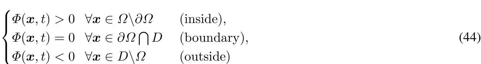
The level set method (LSM) was first proposed by Osher et al. [Osher and Sethian (1988)]to track the evolution of free surfaces in computational fluid dynamics, and has proven to be effective in representing complicated boundaries in a wide variety of applications. In the LSM, the structural boundary ∂Ω is implicitly embedded as the zero level set of a onedimensional-higher level set function (LSF) Φ(x, t), where x is the coordinate vector of a point and t is a pseudo time. The level-set-based topology optimization handles the complex topological changes by the motions of implicit boundaries represented by the LSF Φ(x, t) which is defined over a reference domain D ⊂ Rd(d = 2 or 3). The level set representation of the structure is defined as

Differentiating the LSFΦ(x,t)with respect to the pseudo-time t,the Hamilton-Jacobi equation is obtained as[Wang,Wang and Guo(2003)]

where the normal velocity vnis

The Hamilton-Jacobiequation Eq.(45)defi nesan initial valueproblem for thetimedependent functionΦ.In the optimization process,vnis the movement of a point on a surface driven by theobjectivefunction of theoptimization,and theoptimal structural boundary is obtained by solving Eq.(45).

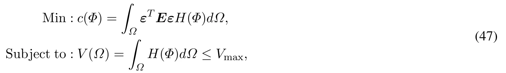
A level-set-based topology optimization for theminimum compliancedesign problem may be defi ned mathematically as[Wang and Benson(2016a)]

where H(Φ)isthe Heaviside function defi ned as

Figure12:Thelevel-set-based ITOof the Michell typestructures:(a)Design domain without geometric constraint,(b)Design domain with geometric constraint,(c)Optimization result without geometric constraint and(d)Optimization result with geometric constraint[Wang and Benson(2016b,a)]

c is the compliance,E is the elasticity matrix andεis the strain.The inequality V(Ω)≤Vmaxdefinesthevolumeconstraint.

To avoid solving the Hamilton-Jacobiequations,Wang et al.[Wang and Benson(2016b)]used the NURBSbasisfunctionsto represent the LSFin aparameterized modeas

where φi(t) is the i th expansion coefficient and Ni(x) is the corresponding basis function.After this parameterization, the LSF associated with both space and time is divided into the spatial terms Ni(x) and the time dependent terms φi(t), and only the latter are updated during the optimization procedure.

The same NURBS basis functions were also used to evaluate the objective function in the level-set-based isogeometric topology optimization (ITO) proposed by Wang and Benson[Wang and Benson (2016b)]. They later extended the level-set-based ITO to solve geometrically constrained problems using trimmed elements [Wang and Benson (2016a)].According to the work of Wang and Benson, using IGA to replace FEM can accelerate the optimization more than 3 times when quadratic elements are utilized and make the optimization iterations easier to converge. Fig. 12 shows the optimization results for the geometrically constrained and the classical Michell type problems.

Figure 13: The level-set-based ITO of the L-shape structure: (a) Design domain and boundary conditions, (b) Initial topology, (c) Optimization result and (d) Von Misses stress contour [Ghasemi, Park and Rabczuk (2017)]

J ahangiry et al. [Ghasemi, Park and Rabczuk (2017)] proposed a similar level-setbased ITO where the LSF is parameterized using NURBS basis functions, and applied the level-set-based ITO to a series of problems including minimizing the mean compliance with a material volume constraint, minimizing weight with consideration of reducing local stress concentration, and simultaneously minimizing the weight and strain energy considering local stress constraints. An L-shape structure with stress constraint that is optimized by the proposed method is given in Fig. 13.

With the help of the high-continuity of IGA, the ITO is able to solve some problems that may be very difficult for the conventional topology optimization using FEM. For example,Ghasemi et al. [Ghasemi, Park and Rabczuk (2017)] presented a level-set-based ITO of flexoeletric materials, which requires at least C1continuous approximations because of the fourth order partial differential equations (PDEs). The proposed ITO is also able to noticeably increase the electromechanical coupling coefficient, with substantial enhancements observed for higher aspect ratios.

Figure 14: Numerical examples of the ITO using the phase field m odel: (a) Design domain of the 2D example, (b) Design domain of the 3D example, (c) Design domain of the thin shell example, (d) Optimization result of the 2D example, (e) Optimization result of the 3D example, and (f) Optimization result of the thin shell example [Dedè, Borden and Hughes(2012)]

4.3 Other types of isogeometric topology optimization

Besides density-based and level-set-based topology optimizations, the IGA can also be integrated with other types of topology optimization methods. Dedè et al. [Dedè, Borden and Hughes (2012)] used IGA for topology optimization with a phase field model in which the optimal topology is obtained as the steady state of the phase transition described by the generalized Cahn-Hilliard equation, and the IGA for the spatial approximation encapsulating the exactness of the representation of the design domain and is particularly suitable for the analysis of phase filed problems. The proposed method has solved both two and threedimensional topology optimization problems and some of the results are shown in Fig. 14.Recently, Guo et al. [Guo, Zhang and Zhong (2014); Zhang, Yuan, Zhang et al. (2016)]developed an explicit topology design optimization approach using the concept of moving morphable components (MMC). The basic idea of this method is based on that arbitrary complicated topology can be decomposed into a finite number of components and the desired topology structure can be obtained by optimizing the central position, length,inclined angles, and some other geometrical features of components. In the MMC topology optimization, a component with straight skeleton and quadratically variable thicknesses (i.e. the i th component) can be described by a set of geometric parameters consisting of coordinates of center, half length, variable thicknesses and inclined angle as Di= (x0i, y0i, Li, t1i, t2i, t3i, θi), and the detail meaning is shown in Fig. 15. Based on these geometric parameters, the structural topology can be explicitly and uniquely described by a vector of design variables D = (DT, D2T, ..., DnT)T.

Figure 15: Geometry description of the i th component with straight skeleton and quadratically variable thicknesses [Xie, Wang, Xu et al. (2018)]

Hou et al. [Hou, Gai, Zhu et al. (2017)] first proposed an explicit ITO using IGA to perform the MMC-based topology optimization, which not only explicitly preserve the geometric and mechanical information in topology optimization, but also provides a more fl exible process for analysis and optimization. However, there is an imperfection of both conventional MMC-based topology optimization and MMC-based ITO that the overlapped region of components is dealt with by the max function with only C0continuity, which results in the objective function becoming nondifferentiable and may cause a low convergence rate of optimization. To overcome the C1discontinuity problem, Xie et al. [Xie, Wang, Xu et al.(2018)] used the differentiable R-function [Shapiro (1991)] to replace the max function and proposed a new MMC-based ITO. Besides, they also presented three new ersatz material models based on uniform, Gauss and Greville abscissae collocation schemes to represent both the Young’s modulus of material and the density fi eld based on the Heaviside values of collocation points, and successfully solve both 2D and 3D optimization problems (see Fig. 16).

Figure 16:Numerical examples of the MMC-based ITO:(a)Design domain of the 2D example,(b)Initial designof the2Dexample,(c)Optimizationresultof the2Dexample,(d)Design domain of the3Dexample,(e)Initial design of the3Dexampleand(f)Optimization result of the3D example[Xie,Wang,Xu et al.(2018)]

5 Conclusions and research trend

In this work, the development of a decade of isogeometric design optimization is comprehensively reviewed with proper comparisons to traditional FEM-based design optimization.Attention is focused on shape and topology optimizations, with size optimization briefl y covered in between.

For isogeometric shape optimization, the typical parameterization problems in FEM-based shape optimization can be avoided due to the seamless CAD-CAE integration framework,however, analysis-suitable parameterization methods for designing complicated geometries become the new challenges, which has been intensively studied in the past few years(see Section 3.1). Although the exact geometry representation of isogeometric framework averts the problem of jagged boundary in FEM-based shape optimization, proper boundary and domain mesh regulation methods are still necessary to ensure the stability of the optimization process (see Section 3.1.3). Isogeometric shape optimization also reduces the difficulties of computing derivative terms with respect to design parameters, leading the direct differential method for shape sensitivity analysis to be popularly used (see Section 3.2).

The seamless CAD-CAE integration framework also promote the development of structural designs with increasingly complicated geometries. Novel software platforms with highly integrated design-analysis engines are becoming more practical and achievable, which will be a great revolution for computer added design technologies.

Currently, shape design for curved structures with special applications using IGA is of great interest, e.g. using isogeometric shape optimization to design auxetic structures with smoothed features in Wang et al. [Wang, Poh, Dirrenberger et al. (2017); Choi and Cho(2018b); Weeger, Narayanan and Dunn (2018)], which focuses on the design of lattice structures with enhanced properties by exploring possible curved unit structures. Combining the finite cell method (FCM) [Guo and Ruess (2015)] with isogeometric analysis for designing curved structures with openings (e.g. in He et al. [He, Pan, Zou et al. (2014)]) or further apply it to topology optimization (e.g. in Cai et al. [Cai, Zhang, Zhu et al. (2014);Zhang, Zhao, Gao et al. (2017)]) is also interesting as it promotes the isogeometric design optimization to be applied to geometrically complicated structures. With the development of analysis-suitable parameterization methods, proper design platforms integrating these new methods for industrial applications would also be interesting. As the IGA has such unique advantages in both analysis [Hughes, Cottrell and Bazilevs (2005)] and design, it should be used to promote the development of challenging problems, e.g. design optimizations for time-dependent, nonlinear solid and fluid mechanical problems. The convenience and efficiency of both geometry and analysis modeling can help to improve global optimization algorithms, which are becoming increasingly practical and favorable (see Haftka et al. [Haftka (2016); Haftka, Villanueva and Chaudhuri (2016)]).

The integrated design-analysis framework in IGA averts the manual transition effort from a CAD model to a FE model, which makes it possible to perform large amount of analysis automatically by varying the geometry design parameters. This is relatively advantageous in the age of big data. With massive results, data-driven design for structural optimization can become increasingly applicable and useful [Queipo, Haftka, Shyy et al. (2005); Forrester and Keane (2009); Xu, You and Du (2015)]. Hence, developing proper methods integrating surrogate modeling, e.g. in Benzaken et al. [Benzaken, Herrema, Hsu et al. (2017)],and artificial intelligence using IGA should also be encouraged to benefit the engineering industry and human society.

For isogeometric topology optimization (ITO), the advantages of IGA has been successfully integrated into topology optimizations. For example, the local support property can free the checkerboards, better efficiency for high order elements greatly increase the efficiency of topology optimization with high-order elements, and the high continuity property can easily solve topology optimizations requiring high continuity, such as the Kirchhoff plate optimization and flexoeletric material optimization. In the future, the IGA will be extended to solve more topology optimization problems, especially for the problems which are impossible or very difficult to complete by conventional topology optimizations. Some of the ITO research trends are summarized hereinafter.

The IGA with high continuity and accuracy is suitable for shell topology optimization, especially for the shell with curved boundary and the curved shell in 3D space [Benson,Bazilevs, Hsu et al. (2010, 2011); Lei, Gillot and Jezequel (2018a)]. Since the shell structures are widely used in the engineering domains such as aerospace, vehicle and ship, the ITO for shell structure optimization has a bright prospect for solving engineering problems.Moreover, the IGA has the local refinement ability [Vuong, Giannelli, Jüttler et al. (2011);Scott, Li, Sederberg et al. (2012); Wu, Huang, Liu et al.(2015)], which provides an opportunity to easily implement the topology optimization with adaptive mesh [Lambe and Czekanski (2018); Wang, Kang and He (2013)]. Definitely, the ITO can be also combined with other approaches used in conventional topology optimizations, e.g. Shepard interpolation [Xia and Shi (2018)], size control approach [Zhou, Lazarov, Wang et al. (2015)], etc.,and extend its application for more physical domains such as thermoelasticity [Xia, Xia and Shi (2018)], fluid-structure interaction [Jenkins and Maute (2015)] and thermal-fluid flow[Yaji, Yamada, Yoshino et al. (2016)].

Besides, Topology optimization has demonstrated its great potential in designing architectured materials with tunable properties since 1980s [Sigmund (1994, 1995)]. The effort of designing such materials in a concurrent multiscale levels is gaining renewed interests, e.g.in Abdalla et al. [Abdalla, Setoodeh and Gürdal (2007); Wang, Abdalla and Zhang (2017,2018); Wang, Abdalla, Wang et al. (2018)] for designing composite laminate with tailored local properties; in Xia et al. [Xia and Breitkopf (2014a,b); Da, Cui, Long et al. (2017); Da,Yvonnet, Xia et al. (2018); Wang, Arabnejad, Tanzer et al. (2018); Wu, Xia, Wang et al.(2019)] for general lattice structures designs. Such work can been extended in the context of isogeometric analysis and will become a new research trend.

Acknowledgement:This work was supported by National Natural Science Foundation of China (51705158), the Fundamental Research Funds for the Central Universities (2018MS45), and Open Funds of National Engineering Research Center of Near-Net-Shape Forming for Metallic Materials (2018005).