ZHU Zichen (朱子晨), WANG Yongzhi (王勇智) , BIAN Shuhua (边淑华),HU Zejian (胡泽建), LIU Jianqiang (刘建强), LIU Lejun (刘乐军)

The First Institute of Oceanographic, State Oceanic Administration, Qingdao 266061, China

Abstract We modi fied the sediment incipient motion in a numerical model and evaluated the impact of this modi fication using a study case of the coastal area around Weihai, China. The modi fied and unmodi fied versions of the model were validated by comparing simulated and observed data of currents, waves, and suspended sediment concentrations (SSC) measured from July 25th to July 26th, 2006. A fitted Shields diagram was introduced into the sediment model so that the critical erosional shear stress could vary with time. Thus, the simulated SSC patterns were improved to more closely re flect the observed values, so that the relative error of the variation range decreased by up to 34.5% and the relative error of simulated temporally averaged SSC decreased by up to 36%. In the modi fied model, the critical shear stress values of the simulated silt with a diameter of 0.035 mm and mud with a diameter of 0.004 mm varied from 0.05 to 0.13 N/m 2, and from 0.05 to 0.14 N/m 2, respectively, instead of remaining constant in the unmodi fied model.Besides, a method of applying spatially varying fractions of the mixed grain size sediment improved the simulated SSC distribution to fit better to the remote sensing map and reproduced the zonal area with high SSC between Heini Bay and the erosion groove in the modi fied model. The Relative Mean Absolute Error was reduced by between 6% and 79%, depending on the regional attributes when we used the modi fied method to simulate incipient sediment motion. But the modi fication achieved the higher accuracy in this study at a cost of computation speed decreasing by 1.52%.

Keyword: sediment model; incipient motion; suspended load; critical shear stress for erosion; fraction of mixed grain size sediment

1 INTRODUCTION

In coastal marine areas, sediment transport has a considerable in fluence on both the natural environment and human activities, such as navigation and marine engineering (Chen et al., 1999, 2004). Environment protection strategies for the coastal zone are often based on the findings from numerical modeling,rather than direct monitoring data as it is generally very difficult and expensive. It is, however, very difficult to simulate natural sediment transport processes because of their complexity. The main sources of suspended sediment in sea water are the erosion mass flux and river inputs. In this study,incipient motion refers to the critical erosional shear stress and the erosion mass flux of mixed grain size sediment, both of which vary temporally and spatially,and are used as constant parameters in most ocean models. In general, the conditions for incipient sediment motion are not fully re flected in numerical models, and the model simpli fication may result in extremely inaccurate simulations.

Spatial variation of incipient motion has been extensively studied. Ge et al. (2015) proposed a method for estimating the critical erosional shear stress that combines a model with GOCI remote sensing data and is suitable for determining spatial variations in the erosion conditions. However, high resolution remote sensing data are not always available. The distribution of sediment with different properties and sizes on the seabed has more in fluence on spatial variations in incipient sediment motion than the distribution of the critical sheer stress.Yamashita et al. (2009) statistically classi fied the grain size distribution of the seabed sediment, and used a sediment trend model to estimate the sediment transport pathways. Schmelter et al. (2015) developed a multi-fraction Bayesian sediment transport model that considered sediment as mixed grain-size components instead of a single component. Using another method to represent spatial variation of incipient motion. Warner et al. (2008) added an unlimited number of de fined non-cohesive sediment classes to the model. Each class had a unique grain diameter, density, settling velocity value, critical erosion stress threshold, and erodibility constant. This approach accounts for spatial variation in the incipient motion if the attributes of the sediment classes change.Sediment consists of gravel, sand, silt, and mud, and there can be considerable spatial variation of the fractions of the components. Instead of classifying the grain-size distribution, we suggest that the fractions of different grain size sediments should be used to re flect spatial variation in incipient motion in our model.

We consider that the critical erosional shear stress can represent temporal variations of incipient sediment motion. In the marine environment, the critical shear stress is a function of the Reynolds particle number, which is not constant in time.Temporal variations in the critical stress can be calculated using the Shields diagram. For example,Bui et al. (2005) used the Shields diagram to determine the critical bed shear velocity for sediment motion in their model, and Health et al. (2015) showed that the shear stress was a function of the speed, and the fluid and particle densities. The critical stress is often estimated from the empirically-based Shield diagram,which relates a dimensionless parameter of critical shear stress to the Reynolds number. Although the Shields diagram has been used to determine the critical shear stress for erosion in previous model studies, temporal variations have not yet been included in a numerical model. In our study, therefore,we introduced the Shields diagram fitted by Dai et al.(2014) into the model to calculate the instantaneous critical shear stress at every time step, and allowed it to vary with time.

The remainder of the paper is organized as follows.In Section 2, we describe the calculation of sediment incipient motion, including the temporally varying critical shear stress for erosion and the spatially varying fraction of mixed grain size sediment. In Section 3, the modi fied numerical model and three comparison models are applied to the Ningjin marine area in Weihai, China, to illustrate the improvement provided by our method. The simulation results of the modi fied and comparison models are compared with observations, and the improvement is evaluated in Section 4. Finally, the conclusions are summarized in Section 5.

2 METHOD

2.1 Model improvement

Our model improvement is based on the unstructured-grid, 3-D, primitive equations FVCOM(Chen et al., 2013), which was developed by a joint research team of the University of Massachusetts Dartmouth (UMassD) and Woods Hole Oceanographic Institution (WHOI). Meanwhile, wave simulation is based on the surface wave model SWAN (Simulating Waves Nearshore). SWAN was developed originally by Booij et al. (1999) and improved by the SWAN Team (2006). The FVCOM development team has converted the structured-grid surface wave model SWAN to an unstructured-grid, finite-volume version under the FVCOM framework (Chen et al., 2013).

The FVCOM sediment module uses a concentration-based approach subject to the following evolution equation:

where t is time; x, y, and z are the east, north, and vertical axes in the Cartesian coordinate system; and u, v, and w are the x, y, and z velocity components,respectively; c is the suspended sediment concentration(SSC); Ahis the horizontal eddy viscosity; Kmis the vertical eddy viscosity coefficient. The settling velocity wsis set by the user for each sediment type.At the surface, a no- flux boundary condition was used for the sediment concentration:

where ζ is the height of the free surface. At the bottom,the sediment flux is the difference between deposition and erosion:

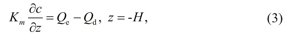
where H is the water depth; Qdis deposition mass flux; and Qeis erosion mass flux.

For the sediment incipient motion discussed in our study, we refer to the critical shear stress for erosion( τce) and the fractions ( f) of mixed grain size sediment components, which control the erosion rate (Amos et al., 2010; Jacobs et al., 2011; Carniello et al., 2012).τceis the function of sediment diameter, cohesive force and shear stress on the seabed (Berlamont et al.,1993; Lumborg and Windelin, 2003; Pouv et al.,2014). In most of the sediment modules of ocean models (e.g., ECOM, FVCOM, and Mike 21), the critical shear stress or critical velocity for erosion is a constant parameter arti ficially set by users. Thus,incipient motion condition is usually determined by the empirical methods (e.g., Houwing and van Rijn et al., 1998; Houwing 1999; Kim et al., 2000). However,τcevaries with time, which is ignored in the models.Furthermore, sediment type varies with space, which makes both the critical condition and erosion mass flux not uniform in the coastal area. The distribution of the median size ( d50) can be used to re flect the distribution of sediment type (e.g., Yamashita et al.,2009). However, we select to use the distribution of fraction ( f) of each component to re flect the sediment type distribution, because mixed grain size sediment components are simulated in our model.

2.1.1 Temporally varying critical shear stress

In the FVCOM sediment module, the erosion mass flux is calculated using the equation (Ariathurai and Arulanandan, 1978) as

where meis the erosion rate, which represents the erosion mass flux in unit time and unit area; τ is the shear stress on seabed for combined waves and currents, and calculated in the hydrodynamic module of FVCOM; τceis the critical shear stress for sediment erosion; and f is the fraction of each sediment component.

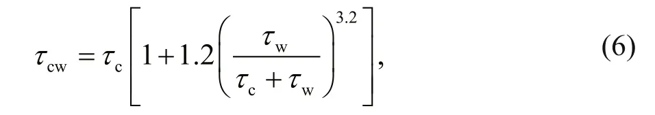
The bottom stress for the combined dynamic of waves and currents in FVCOM is computed using the parametric approximation by Soulsby and Whitehouse(1997).

where τwis the amplitude of shear stress due to waves without currents and α is the angle between the currents and waves. τcwis the combined waveaveraged stress in the current direction and is calculated as

where τcis the shear stress due to currents without waves. The amplitude of shear stress due to waves without currents ( τw) is calculated as

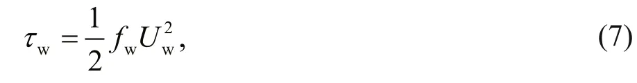
where fwis the wave friction factor and Uwis the bed wave orbital velocity.

In the present sediment module of FVCOM, the critical shear stress for erosion is a constant parameter.Until now, critical shear stress has been widely discussed with respect to its in fluencing factors, such as, diameter and cohesion (e.g., Andersen et al., 2007;de Linares and Belleudy, 2007; Ge et al., 2015).Critical shear stress is the function of the particle Reynolds number, which is in fluenced by the current.The fitted Shields diagrams (e.g., Kennedy, 1995;Buffington, 2000; Cao et al., 2006; Dai et al., 2014)can be introduced into a numerical model to calculate the critical shear stress autonomically. The previous studies illustrated that Shields diagram is suitable for sand, silt and mud. The fitted diagrams proposed by previous studies all show that the relative critical shear stress for erosion ( θce) reaches the minimum value when the Reynolds number is close to 10. When the Reynolds number is larger than 10, θceincreases as the Reynolds number increases. Conversely, when the Reynolds number is smaller than 10, θcedecreases as the Reynolds number increases.

Dai et al. (2014) proposed a fitted Shields diagram using a probabilistic method. The functional relationship between the relative critical shear stress for sediment erosion and the particle Reynolds number is given by the fitted Shields diagram as

where Re*is the particle Reynolds number; ρsis the density of sediment; and θceis the relative critical shear stress for sediment erosion. θcecan also be expressed as

where τceis the critical shear stress for sediment erosion in the model; γ and γsare unit weights of seawater and sediment, respectively; d is the sediment diameter. Combining Eqs.8 and 9, τcecan be calculated with Re*as follows

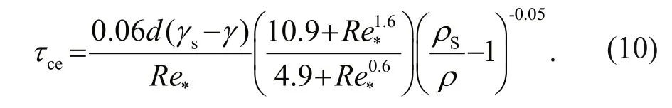
Furthermore, Re*is the function of friction velocity,given as

where υ is the kinematic viscosity coefficient; and U*is the friction velocity, which is the function of shear stress.

In Eq.12, τ is the shear stress on seabed. Combining Eqs.11 and 12, Re*is the function of τ, and thus varies with time, as follows

Instantaneous τcecan be calculated by combining Eq.10 with Eq.13. And τ can be calculated in the hydrodynamic module of FVCOM using Eq.5.

2.1.2 Settling flux

As we focus on suspended load (silt and mud) and the grain size is smaller than 0.1 mm in our study, the settling velocity of each component is calculated with the Stokes formula, given as

where g is acceleration due to gravity.

Prandle (1997) proposed that the assumption of settlement at the rate Qd= wscb( cbis SSC at the bottom)is generally twice the value pertaining for a Gaussian vertical sediment distribution (with null position centered at - wst relative to the bed) with dispersion counteracting half of this advective settlement. Thus,the depositional velocity can be de fined (Prandle,1997) as

where wdis the depositional velocity at the bottom.Then, the deposition mass flux is calculated as

2.1.3 Spatially varying fraction

As discussed above, sediment type is not uniform in space. In the present FVCOM, mixed grain size sediment has already been introduced. However, the spatially-dependent components are not re flected.Different sediment components have different fractions ( f) in the coastal area, and the fraction represents the areal percentage of a particular sediment component in a unit area. By interpolating the fraction of each individual sediment component into each element as an input condition for the model,the spatially-dependent erosion mass flux can be determined.

In FVCOM, the unstructured triangle grid is comprised of three nodes, a centroid, and three sides,in which the current velocities ( u and v) are placed at centroids and all scalars are placed at nodes. The suspended sediment concentration (SSC) is calculated at the node and determined by the net flux through the sections linked to centroids and the middle point of the sideline in the surrounding triangles (Chen et al.,2006, 2013; Ge et al., 2012). According to this strategy, each sediment component fraction ( f) is set at the node in our modi fied model.

It should be point out that the spatially varying fractions of the mixed grain size sediment also in fluence the drag efficiency from the sediment bed to the bottom current. The functional relationships between the drag coefficient and sediment properties are difficult to determine because of the complex factors, such as, sediment grain size, composition proportion, and viscosity. The bottom roughness parameter and drag coefficient are therefore simplified as uniform in our study. This may cause some inaccuracies in the calculation of the current, which could be propagated into the SSC computation.

2.2 Field experiment

(1) Current, wave and SSC

To judge whether the modi fication improves simulation accuracy, the modi fied and comparison models were applied to simulate a case from nature,and the results were validated with observed data. The experiment deployment took place in the Ningjin marine area, on the coastal zone in Weihai, China(Fig.1).

Fig.1 Locations of observation stations and bathymetry

Four observation stations (marked as D1–D4 in Fig.1) were set up to measure current velocity and SSC from 8:00 on 25thto 9:00 on 26thJuly, 2006. A synchronous wave station were arranged and marked as DW. The current and SSC were measured in five layers. Current velocity was measured with Aanderaa RCM9 Current Meter. SSC was captured with the water sampler and analyzed in laboratory. The bathymetry is shown in Fig.1. The stations were all located in the shoal area with depths less than 20 m,and the survey region was in fluenced by wave action(Chao et al., 2008). Tide and wave height were respectively measured at Stations D3 and DW during 24thto 26thJuly. Tide was measured with a water level indicator and wave height was measured with a Wave Rider Buoy. Measurement interval was 1 h. The observation was conducted during the spring tide period.

(2) Particle size

Fig.2 Compositions of bottom and suspended sediment, and distribution of sediment type

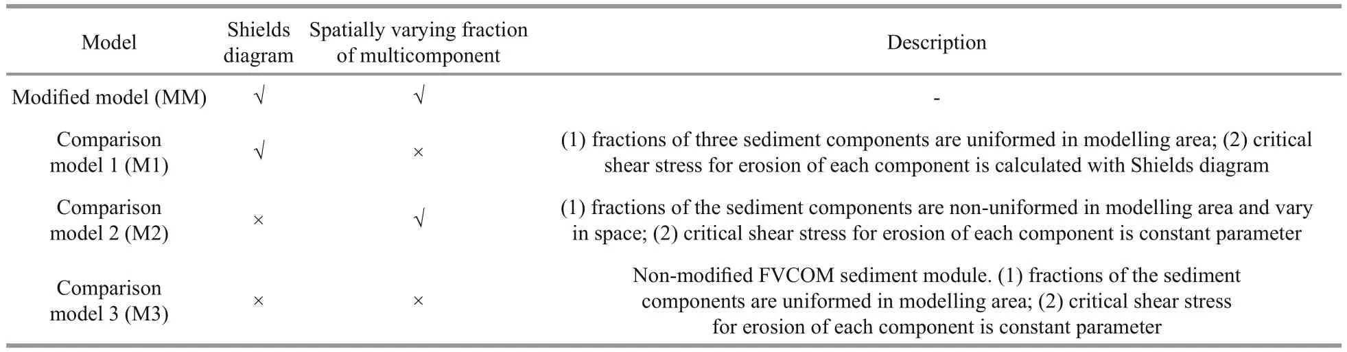
Table 1 Settings of the modi fied model and the comparison models

Grain sizes of bottom material on seabed at the observation stations were analyzed (Fig.2b). The bottom material at D1 and D3 mainly consists of bed load sediment, with 99.9% of the sediment consisting of the mixture of sand and gravel. 92.4% of the sediment are sand at D3. This laboratory experimental analysis result is consistent with the survey result(Fig.2a) by State Oceanic Administration (SOA) et al.(1990). And the percentage compositions in Heini Bay are similar to the study by Yin et al. (2013). As we focus on suspended load sediment, and because of the less native erosion mass flux at D1 and D3, the grain sizes of suspended sediment were analyzed at Stations D2 and D4. Laboratory analysis shows that the suspended particle diameters vary from less than 0.001 mm to 0.063 mm. The percentage compositions of different suspended sediment size grades are displayed in Fig.2c. Because the median grain size of suspension varies non-signi ficant in a tidal cycle(Bian et al., 2017), the statistics were analyzed at four individual moments, which were 12:00 (12:00 at D1 and 11:30 at D3), 15:30, 19:30, and 23:00 on July 25th, 2006.

2.3 Model settings

To explain the improvement of the modi fied model,the effects of introducing the Shields diagram and the spatially varying fraction of mixed grain size sediment were analyzed by comparing with the unmodi fied FVCOM and two half-modi fied models. The settings of the four models are listed in Table 1. The Shields diagram and the spatially varying fraction were both introduced into our modi fied model (marked as MM).In comparison model 1 (marked as M1), only the Shields diagram was introduced to evaluate how the accuracy was improved by the spatially varying fraction of the mixed grain size sediment. In comparison model 2 (marked as M2), only the spatially varying fraction was introduced to show how the accuracy was improved by introducing the Shields diagram. Comparison model 3 (marked as M3) was the unmodi fied FVCOM. The simulation period was from 0:00 on 23thto 23:00 on 26thJuly,2006, which contains the observation period.

(1) Mesh and boundary conditions

Fig.3 Enlarged view of calculation meshes

To improve the precision of our model, the meshes were subtilized and displayed in Fig.3. The horizontal resolution varied from 0.15 km around the study area,to 5 km along the lateral boundary and near the open boundary. The water column was divided into 20 layers in the 3-D model. The local domain FVCOM was driven by eight major astronomical tidal constituents- M2, S2, K2, N2, K1, O1, P1, and Q1-through nesting with the regional coastal FVCOM at the outer open boundary. Wind field data from the National Oceanic and Atmospheric Administration, U.S.(NOAA) was used to simulate the wave field over a larger region. The wave field results were then added into the model as boundary conditions in a subtilized area.

(2) Spatially varying fractions

The grain size analysis results show that the grain size varies from less than 0.001 mm to 0.063 mm(Fig.2c). In our model, two types of sediment components, silt ( d=0.035 mm) and mud( d=0.004 mm), were simulated. The silt component was used to represent the sediment with diameter varying from 0.008 mm to 0.063 mm, and the mud component represented the remaining sediment components (0.001 mm to 0.008 mm).

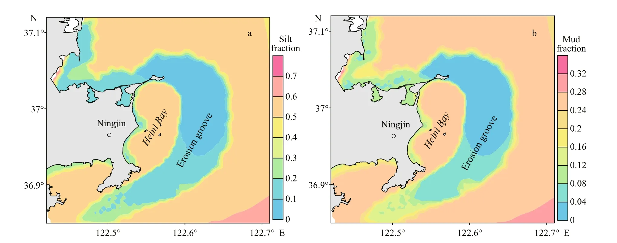
Fig.4 Fraction settings distributions of each simulated component in modi fied model (MM) and comparison model 2 (M2)

As shown in Fig.2a, the sediment type on seabed varies signi ficantly in space. Due to the effect of wave action, sediment in the nearshore region mainly consists of sand. The dominant sediment component changes to be the mixture of silt and mud in Heini Bay. In the erosion groove with depths exceeding 20 m (Fig.1b), sand and even gravel are the primary components. The fractions of the two simulated components are determined by the observations and interpolation by Yin et al. (2013) and Yin (2013) in Heini Bay with 75 stations survey of seabed material.In Heini Bay, silt percentage composition is varying from 50.8% to 82.4%, and mud percentage composition is varying from 15.5% to 35.2%. In the nearshore zone with depth less than 5 m, more than 92.4% of the sediment are sand. The fractions in the erosion groove are arti ficially set by referring to the survey result by SOA et al. (1990), and calibrated with our observation data. The fractions of the two simulated components are shown in Fig.4. As the fractions of the silt and mud components were interpolated into the meshes, the sum of the fractions of the two components could be less than 1. The remainder was therefore the fraction of the bedload component (gravel and sand), which is hard to start.The fractions of the two components were de fined as 0.65 and 0.30 in comparison model 1, which was the same as the fraction in the YT region (Fig.2a) in the modi fied model and comparison model 2.

(3) Parameters

The other model parameters are listed in Table 2. In similar modeling studies, the free parameters have been determined by fitting the model results to the observations (e.g., Aldridge, 1996; Jago and Jones,1998; Bass et al., 2002). Some of the parameters in this study were determined by referring to similar studies and calibrating with observational data.

3 RESULT

To de fine whether the simulation accuracy is improved by the modi fications, both the qualitative and quantitative manners were applied. The qualitative manner means validating the simulated hydrograph with the observed. By this manner, validation results could be presented intuitively, and the variation tendency in time could be shown clearly. To quantitatively evaluate the improvement effect, The Relative Mean Absolute Error (RMAE) was applied.RMAE is calculated as follows (van Rijn et al., 2003):

Tide level:

Wave height:

Current speed:

Suspended sediment concentration (SSC):

in which ζc, Hwc, Vc, and Ccare the calculated tide level, current speed, wave height and SSC. ζm, Hwm,Vm, and Cmare the measured tide level, current speed,wave height and SSC. Δ ζm, Δ Hwm, Δ Vm, and Δ Cmare the errors of measured tide level, current speed, wave height and SSC. ＜··＞ means averaging procedure over time series. Δ Hwmis de fined as 0.1 m and Δ Vmisde fined as 5 cm/s according to their measurement instruments and referring to the study by van Rijn et al. (2003). Δ ζmis de fined as 5 cm according to the measurement instrument. Δ Cmis de fined as 5 mg/L according to the measurement method. The absolute difference of the calculated and measured values minus the measurement error cannot be smaller than zero (e.g., | Hwc– Hwm|–Δ Hwmis zero, if＜0). The relative errors will be relatively large, if the average value is close to zero. Therefore, the RMAE can give very high values that are exceptionally sensitive to small perturbations in the average.

Table 2 Main model parameters

3.1 Hydrodynamic validation

The observation results are shown in Fig.5 and represented by the discrete points. The features of the semidiurnal tide were distinct with a tidal range of 2 m in the study area. The current was observed during the spring tide period. The characteristics of the reversing current were obvious.

At the observation stations, the strongest hydrodynamic occurred at Station D1, which was located near the cape with a depth of 10 m. The current speed at maximum flood (94 cm/s) was higher than the speed at maximum ebb (79 cm/s) at D1 during the observation period. At station D4, the duration of the tidal rise was longer than that of ebbtide because of the in fluence of the topography. The weakest hydrodynamic occurred at D3, which was located at the bay head with a depth of 6 m. The current speed reached 30 cm/s at maximum flood, and 26 cm/s at maximum ebb. The study area is strongly in fluenced by wave action with wave directions of NNE, NE, and SE. From 8:00 to 19:00 on 25thJuly,2006, the direction of the dominant wave was NE.From 0:00 to 18:00 on 26thJuly, the study area was markedly in fluenced by wave action with a maximum wave height of 0.6 m, and the direction of the dominant wave was SE. At the wave observation Station DW, three peaks with wave heights higher than 0.4 m occurred at 20:00 on July 25th, 8:00 and 14:00 on July 26th.

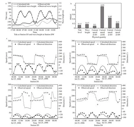
Fig.5 Validation and Relative Mean Absolute Error (RMAE) of tide, wave height and vertically integrated current velocity

The calculated tide is consistent with the measurement result (Fig.5a). The hydrodynamic module of FVCOM produces reasonable results for tide level (RMAE=0.13, in Fig.5b). Referring to the study by van Rijn et al. (2003), the simulation result for wave height is reasonable if RMAE is smaller than 0.2. The result for current speed is good with RMAE smaller than 0.3 and reasonable with RMAE smaller than 0.5. Therefore, the simulation result for wave height is reasonable (RMAE=0.17). The results for current speed are good at station D1 and D4(RMAE=0.10 at D1, RMAE=0.21 at D4), and reasonable at D3 (RMAE=0.45). The wave height at DW and the current velocities at D1, D3 and D4 are slightly different to the observed. Nevertheless, the simulated current speed at D2 was much higher than the observed (Fig.5c). The maximum observed vertically integrated speed was 43 cm/s with the simulated maximum speed of 81 cm/s. The simulation error at D2 is obvious (RMAE=0.95). The difference is mainly caused by the in fluence of raft culture.Although August is not the planting season for seaweed, the rafts are retained and in fluence the current nearby. The flow resisting effect caused by raft could in fluence the 0.8H water layer in the study area (Zhang et al., 2016). As Station D2 is surrounded with culture rafts, by the flow resisting effect from the rafts, the simulated current speed at D2 is much higher than the observed. Recently, the flow resisting effect caused by raft could not be re flected by the model.

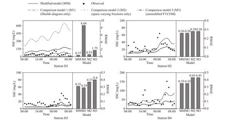
Fig.6 SSC validation of modi fied model (marked as MM) and three comparison models (comparison model 1: marked as M1,Shield diagram only, no spatially varying fractions; comparison model 2: marked as M2, spatially varying fractions of the two simulation sediment components, Shields diagram is not introduced; comparison model 3: marked as M3,unmodi fied FVCOM) and Relative Mean Absolute Error (RMAE) of calculated vertically integrated SSC

The simulation error in hydrodynamic module could cause error in sediment module directly because of the following reasons: 1) the hydrodynamic error would be propagated to shear stress on seabed. As a result, the calculated SSC would be lower with low velocity and wave height, and higher with strong hydrodynamic conditions; 2) as critical shear stress for erosion in the modi fied model is calculated by the Shields diagram, and the Reynolds number is in fluenced by the friction velocity. Thus, the modi fied model is more sensitive to the hydrodynamic error,compared with the unmodi fied FVCOM.

3.2 SSC validation

The sediment transport was basically in a balanced state of erosion and deposition in the study area. The characteristics of the regular semidiurnal tide dominate the area. The current and suspension movement is therefore highly cyclical. The 26 hours observation and validation contained two tidal cycles,and therefore re flect the fundamental regular patterns of the current and SSC movement. In addition, the observation and simulation were conducted during the spring tide to reduce the impact from wave action,as wave movement is fast and wave data with high time resolution is rare. The simulated and observed SSC are compared in Fig.6. As the variation tendencies of surface and bottom SSC are similar to that of vertically integrated SSC, we select vertically integrated SSC to represent the variation process because of its representativeness for the whole water column.

The observed average vertically integrated SSC at Stations D1-D4 during the two tidal cycles were 42,25, 16, and 44 mg/L. The observed maximum vertically integrated SSC at the stations were 117, 64,42 and 151 mg/L. The simulation results of the modi fied model (MM) were the nearest to the observed with average vertically integrated SSC of 51, 25, 8 and 49 mg/L, and maximum vertically integrated SSC of 87, 51, 18 and 90 mg/L at the stations. The SSC hydrograph of comparison model 1(M1) and the hydrographs of MM overlap at D2 and D4. The two stations are both in the YT region (Fig.2a)and the fractions at the stations in M1 are therefore the same as those in MM. As a result, the two models have the same simulation accuracy at D2 and D4. The SSC hydrograph of comparison model 2 (M2) and the hydrograph of comparison model 3 (M3) also overlap at D2, because the fractions were the same, and the critical shear stresses were set as constant in both the models. For the unmodi fied model (M3), the average vertically integrated SSC were 124, 16, 6 and 27 mg/L at the stations, and the maximum vertically integrated SSC were 179, 27, 10 and 42 mg/L. The improvement of the method for simulating sediment incipient motion is con firmed by the comparisons. For M1, the average vertically integrated SSC were 412, 25, 8 and 49 mg/L at the stations, and the maximum vertically integrated SSC were 650, 51, 17 and 90 mg/L. The better results of MM than the results of M1 con firmed that the accuracy in space was improved by introducing spatially varying fractions. For M2, the average vertically integrated SSC were 19, 16, 6 and 27 mg/L at the stations, and the maximum vertically integrated SSC were 27, 27, 12 and 42 mg/L. The better results of MM than the results of M2 con firmed the accuracy in time was improved by introducing Shields diagram into the model.

Particularly, when the critical shear stress for erosion decreased with shear stress and the Reynolds number increased while Reynolds number smaller than 10, the erosion mass flux calculated by Eq.4 was higher, as the fitted Shields diagram was introduced. Therefore, the SSC of M1 was even higher than the result of the unmodi fied model (M3). The SSC were not completely simulated at D3, because the inshore hydrodynamics were not accurately simulated by our model, and the fractions are not completely consistent with the actual conditions. SSC at D2 was markedly in fluenced by wave action from 0:00 to 8:00 on July 26th.

The Relative Mean Absolute Error (RMAE) of MM was signi ficantly lower than the RMAE of M1 except at D3. This means the simulation accuracy was improved by the method of spatially varying fractions,as only Shields diagram was used in M1. However,although the RMAE of M1 were lower than the RMAE of M3 at most of the stations (D2–D4), the simulation error of M1 was excessive at D1(RMAE=8.64). This means that if only the Shields diagram is introduced without sediment type distribution treatment, the simulation accuracy could be extremely low in certain areas. The lower RMAE of MM than the RMAE of M2 explains that the simulation accuracy was improved by introducing Shields diagram, as only spatially varying fractions method was used in M2. The RMAE of MM varied from 0.26 to 0.37 with the RMAE of M3 varying from 0.28 to 1.75. The RMAE of MM were obviously lower at D1, D3 and D4, and slightly lower at D2 than the RMAE of M3. This means the method in modi fied model improved the simulation accuracy. The Relative Mean Absolute Errors were reduced by 6%to 79% at different characteristic stations.

Although the simulation results of the modi fied model re flected the variation tendency of SSC, there was still differences between the simulated and the observed SSC. This difference was mainly caused by the following factors: 1) sediment movement is a complex physical process, which is not completely clear and cannot be simpli fied by equations in ocean models; 2) in marine area, sediment is a mixture of gravel, sand, silt, and mud. However, the mixed grain size sediment was only represented by two idealized components in our model; 3) SSC is signi ficantly disturbed by wave action. Because wind and wave data in high time resolution is difficult to obtain, the SSC hydrograph could not be completely reproduced by the model; 4) the error in the bottom current simulation caused by the simpli fication of the roughness parameter and drag coefficient was propagated into the SSC simulation.

3.3 Percentage composition

Seabed materials at D1 and D3 mainly consist of bed load sediment. Our study is focus on suspended load, and aimed at improvement for incipient motion of suspension. Therefore, percentage compositions at D2 and D4 were analyzed (Fig.2c). Because of the nonsigni ficant variation of median grain size during a tidal cycle (Bian et al., 2017), the analysis was conducted at four characteristic moments, which are the maximum flood, maximum ebb with strong hydrodynamic condition and high and low tide with weak dynamic.

As two sediment components were simulated in our model, the percentage compositions of the components in the modi fied model were also compared with observation data. Two types of sediment components,silt ( d=0.035 mm, represents 0.008 mm to 0.063 mm)and mud ( d=0.004 mm, represents less than 0.001 mm to 0.008 mm), were simulated. Because the two median diameters were arti ficially set to represent two particle size ranges, the simulated variation tendencies of the percentage compositions could not represent the variation tendencies of the diameter ranges, especially for the silt component with a larger diameter range.However, the comparison between the observation percentage compositions and the simulated still could be useful to judge whether the percentage compositions in the marine area were re flected by the modi fied model (Fig.7).

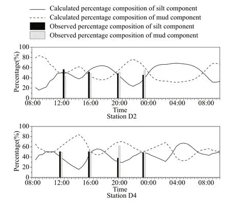
Fig.7 Validation for percentage compositions of simulation components in modi fied model (MM) at Station D2 and D4

The observed percentage composition of the silt fluctuated around 54% (average value) at D2. For the simulated results, the percentage composition of the silt component varied from 16% to 68%, and fluctuated around 48%, which was close to the observed result. The difference occurred because the percentage composition was only observed at four individual moments but simulated during the whole period, and the median diameter was used to represent a range of diameters. The observed percentage composition of the mud fluctuated around 46% with the simulated value fluctuating around 52%. At D4,the observed percentage composition of silt fluctuated around 47% and the simulated varied around 43%.The observed percentage composition of mud component varied around 53% and the simulated varied around 57%.

4 DISCUSSION

4.1 Improvement by spatially varying fraction

(1) Effect at stations

In M1, the spatially varying fraction of mixed grain size sediment was ignored, and only the Shields diagram was introduced. As illustrated in Fig.2b, the bedload component at Stations D1 and D3 was the dominant component of sediment in MM. In M1, the fractions of the sediment components were set as uniform (Table 2) in the whole area. Thus, the calculated SSC was much higher than the observed SSC in the comparison model, and reached 400 mg/L at D1 during the distinct wave action, with the SSC in MM remaining below 150 mg/L.

The silt component experienced more erosion due to its higher rate of erosion (Table 2 and validated in Fig.7) and the lower critical shear stress caused by the larger Reynolds number, which was remaining smaller than 10. There was also a higher deposition mass flux with a higher settling velocity, and the range of variability of the silt component was larger than that of the mud component. The SSC in MM was higher than the SSC in M1 at D2 and D4 when the strong waves occurred on 4:00 on July 26th(Fig.6),because of the higher silt fraction. After the wave action, the SSC in M1 was higher because of the higher mud fraction, which settled slowly.

(2) Effect in horizontal

To explain the inaccuracy caused by ignoring the spatially varying fractions in M1, the horizontal distributions of SSC at four speci fic moments are displayed in Fig.9. The distributions illustrate that the two models have the similar simulation accuracy in the YT regions (Fig.2a). However, in the regions of other sediment types, the accuracy of MM was improved, especially in the SG and MCS regions,where the SSC of M1 was much higher than the SSC of MM, because of larger fractions of silt and mud in M1.

In Fig.9, the simulated SSC by MM in central Heini Bay varied from less than 10 mg/L to 50 mg/L.High SSC range emerged around Heishi Island and the bay head of Heini Bay. SSC in the erosion groove was low, especially at maximum ebb, maximum flood and low tide. Particularly, a high SSC zone emerged between Heini Bay and the erosion groove. The SSC horizontal distribution is similar to previous study in the same area by Liu et al. (2009). In the study by Liu et al. (2009), SSC around Heini Bay was researched by sample survey with 85 stations and remote sensing map (Fig.10). The similar SSC distribution in central Heini Bay (7 mg/L to 30 mg/L), low SSC zone in the erosion groove, and the high SSC zone between the groove and Heini Bay were founded in their study.The high SSC zone between the groove and Heini Bay emerged because of combined effect of current and wave action. The current speed here is higher than the current inside Heini Bay, and the zonal area was in fluenced by wave action signi ficantly.Meanwhile, the groove primarily consists of bedload sediment. Thus, the SSC along the zonal area was higher than the SSC in central of Heini Bay and the SSC in the groove. The nearshore SSC distribution with the depth less than 5 m of our simulation is erroneous with the study by Liu et al. (2009), because of the different wave direction.

Fig.8 Calculated Reynolds number at the given stations in the modi fied model

(3) Effect on the vertical section

To explain the improvement in the accuracy of the 3-D structure, the SSC on a characteristic section is displayed in Fig.11. In the area with depth varying from 20 m to 28 m on this section, the SSC in M1 reached more than 100 mg/L at high tide compared with less than 50 mg/L in MM. The result of MM is closer to the study by Liu et al. (2009). The horizontal and vertical illustrations both show that the spatially varying fractions of the mixed grain size sediment improved the simulation effect in space.

4.2 Improvement by Shields diagram

4.2.1 Calculated critical shear stress

(1) Silt component

The silt sediment component with a median diameter of 0.035 mm began to erode when the shear stress reached 0.13 N/m2, which was calculated using the Shields diagram in our model (Fig.12). As the shear stress increased with current speed, the critical shear stress for erosion decreased and reached a minimum value of 0.05 N/m2. The critical shear stress for erosion measured by Lanuru (2008) varied from 0.11 N/m2to 1.1 N/m2with the grain diameter ranging from 0.02 mm to 0.11 mm. Vanoni (1964) measured relative critical shear stress varying from 0.075 to 0.228 with a grain size of 0.037 mm, which was close to the silt component ( d=0.035 mm) in our model.Critical shear stress was calculated to vary from 0.04 N/m2to 0.13 N/m2, which was similar to our results.

Fig.9 Vertically integrated SSC of modi fied model (MM) and comparison model 1 (M1) at characteristic moments

Fig.10 Surface SSC Remote sensing map by Liu et al. (2009)

Fig.11 Vertically integrated SSC of modi fied model (left panel) and comparison model 1 (right panel) (Shields diagram only)at characteristic section

The Reynolds numbers of the two simulated components are shown in Fig.8. It illustrates that the Reynolds numbers at the stations were less than 2 during the whole calculation period. The Reynolds number of the silt component, which ranged from 0.2 to 1.2, was much larger than that of the mud component with a maximum value of 0.15. This type of phenomenon can be explained with the Shields diagram. Under the condition of Reynolds number smaller than 10, the critical shear stress for sediment erosion ( τce) decreased as the Reynolds number increased. Assuming the shear stress ( τ) on seabed is constant, the Reynolds number of the mud component is smaller than that of the silt component, and the critical shear stress for erosion of mud will be higher than that of silt. For the given simulation components,the critical shear stress for erosion decreased as the current and shear stress increased when the Reynolds number was smaller than 10. As the sediment diameter in our model was less than 0.063 mm, according to the Stokes formula, the settling velocity of the silt component was calculated as 1.06 mm/s. The settling velocity was similar to the velocity calculated by Winterwerp et al. (2006).

Fig.12 Vertically integrated SSC of silt component, shear stress, and critical shear stress of modi fied model (MM) and comparison model 2 (M2)

The phase lag between the shear stress and SSC was also simulated by the modi fied model. The peaks and troughs of SSC occurred occasionally after those of the shear stress. The phase lag occurred because 1)the rapidly varying hydrodynamics did not provide enough time for the bottom/suspended sediment to fully respond. As a result, the peak of SSC did not occur simultaneously with the hydrodynamics(Dohmen-Janssen, 1999; Pritchard, 2005; Xie et al.,2010); and 2) the phase lag can be produced by the combined action of advection, settling, and erosion(Bass et al., 2002).

(2) Mud component

The mud component with a median diameter of 0.004 mm began to erode when shear stress reached 0.14 N/m2, which was calculated using the Shields diagram in our model (Fig.13). As shear stress increased with the current speed, the critical shear stress for erosion decreased and reached a minimum value of 0.05 N/m2. Ge et al. (2015) estimated critical shear stress for erosion in the Changjiang estuary, on the Chinese coast, by combining observations with GOCI remote sensing and modeling. In the area with a diameter less than 0.03 mm, the critical shear stress for erosion varied from less than 0.15 (even close to 0) to higher than 1.8 N/m2, and was in fluenced by regional properties. The values for the critical shear stress for suspension cited in the literature vary between 0.1 N/m2and 0.2 N/m2for mud flats (Williamson and Ockenden, 1996; Lund-Hansen et al., 1999). The critical shear stress for erosion calculated with the Shields diagram in our model was fitted to the previous studies. According to the Stokes formula, the settling velocity of the mud component was calculated as 0.014 mm/s. This is comparable with the previous study by Fettweis (2008), who suggested averages for the settling velocities of mud between 0.003 mm/s and 0.20 mm/s. The settling process of the mud component was relatively slower than that of the silt component.Thus, the SSC of the mud component increased rapidly due to strong wave action from 0:00 on July 26th(Fig.14), and decreased slowly.

Fig.13 Vertically integrated SSC of mud component, shear stress, and critical shear stress of modi fied model (MM) and comparison model 2 (M2)

4.2.2 Improved accuracy

In comparison model 2 (M2), only the method of spatially varying fractions were applied, and the Shields diagram was not included. As explained in Section 2, the Shields diagram re flects the temporally varying critical shear stress for erosion. Thus, by comparing with M2, the improved temporal accuracy of MM can be demonstrated. In the validation curves shown in Fig.6, the SSC calculated by M2 was lower than the observed SSC and the SSC calculated by MM. The low SSC rangeability in M2, which was caused by constant critical shear stress, accounts for the low SSC. To explain the generation mechanism of this low rangeability, the SSC of each simulation component was separated from the total SSC(Figs.12–13). The relationship between shear stress and critical shear stress for erosion was displayed in the figures at the same time. As shown in Fig.12, the critical shear stress of the silt was constant in M2, and equaled the critical shear stress in MM when the silt component began to erode (intersection of shear stress and critical shear stress for erosion in MM and M2).However, as the current speed and shear stress on the seabed increased, the critical shear stress calculated by the Shields diagram decreased in MM, whereas the critical shear stress was constant in M2. As a result,the erosion mass flux in MM was higher than that in comparison model 2 (Eq.4), specially at maximum flood or ebb. Thus, the rangeability in MM is higher than that in M2, and was closer to the realistic value.

In Fig.13, the critical shear stress for the erosion of the mud was constant in comparison model 2, and equaled the critical shear stress in MM when erosion began. The same as in the silt component, the erosion mass flux in MM is higher than that in M2, and the SSC rangeability in MM was higher than that in M2.In particular, when the coastal area was signi ficantly in fluenced by wave action (from 0:00 to 8:00 on July 26th), the shear stress on seabed increased markedly.

At Stations D2 and D4, seabed material mainly consists of silt and mud. Therefore, native erosion mass flux is high. At D2, the observed rangeability of vertically integrated SSC is 55 mg/L with an average SSC of 25 mg/L during the simulation period. The rangeability simulated by MM is 31 mg/L with an average SSC of 25 mg/L. The rangeability simulated by M2 is 12 mg/L with an average SSC of 16 mg/L. At D4, the observed rangeability of vertically integrated SSC is 135 mg/L with an average SSC of 44 mg/L.The rangeability simulated by MM is 64 mg/L with an average SSC of 49 mg/L. The rangeability simulated by M2 is 22 mg/L with an average SSC of 27 mg/L.Compared with simulation results by M2, both the average SSC and the rangeability simulated by MM are closer to the observed values. By introducing Shields diagram into the model, the relative error of simulated SSC rangeability decreased by up to 34.5%,and the relative error of simulated average SSC during two tidal cycles decreased by up to 36%.

4.3 Advantages and disadvantages

(1) Advantages

As discussed above, the main advantage of introducing our method for simulating sediment incipient motion into sediment model is that the simulation accuracy is improved. The Relative Mean Absolute Errors of the modi fied model were reduced by 6% to 79% at the validation stations in our study case. Besides, the accidental error caused different modelers could be avoided, and the automation level of the model is also heightened. The critical shear stress for erosion and particle size of the sediment are arti ficially set by the modelers with different research experience. By introducing the fitted Shields diagram, only the particle size need to be set. Then the critical shear stress could be automatically calculated by the model.

(2) Disadvantages

In our study case, the meshes consisted of 6 224 nodes and 12 034 cells. In the serial computation process with Intel dual-core 1.66 GHz CPUs, the averaged computation speed is 4.98 steps each second, instead of 5.06 steps each second before the modi fication. The modi fication method achieved the advantages of high accuracy at a cost that computation speed decreased by 1.52%. In addition, the critical shear stress for erosion cannot always be easily de fined by Shields diagram because sediment is a mixture. Sometimes, the critical shear stress need to be arti ficially set according to the sediment properties.Although the automation level of the model is heightened by introducing Shields diagram, the flexibility of parameter settings is brought down.

5 CONCLUSION

The critical shear stress for erosion in the sediment transport model was modi fied to vary in time by introducing a fitted Shields diagram. The calculated critical shear stress of the simulated silt component with a diameter of 0.035 mm varies from 0.05 N/m2to 0.13 N/m2, and that of mud with a diameter of 0.004 mm varies from 0.05 N/m2to 0.14 N/m2, instead of remaining constant in the unmodi fied model. Thus,the simulated variation tendency of suspended sediment concentration was modi fied to get closer to the observed. The relative error of the simulated variation range of suspended sediment concentration decreased by up to 34.5% during the spring tidal cycles. And the relative error of simulated temporal average suspended sediment concentration decreased by up to 36%.

The method of applying spatially varying fractions of the mixed grain size sediment enhanced the spatial simulation accuracy over the coastal area where the sediment type on the seabed varied signi ficantly in space. In the study case, the simulated suspended sediment concentration distribution is approximate to the remote sensing map. And the high concentration zone between Heini Bay and the erosion groove was reproduced.

By the method for simulating sediment incipient motion in the modi fied model, the Relative Mean Absolute Error was reduced by 6% to 79% depending on the regional attributes. But the modi fication method achieved the advantages of high accuracy at a cost that computation speed decreased by 1.52% in the study case.

6 DATA AVAILABILITY STATEMENT

The data that support this study are available from the corresponding author upon reasonable request but not for all due to relevant data protection for nuclear power plant security.

7 ACKNOWLEDGEMENT

The authors appreciate the helpful comments and suggestions provided by Mr. CHI Wanqing and Doctor ZENG Ming. The advices helped us with improving this paper.