Dong-mei Ju (剧冬梅), Chang-le Xiang (项昌乐) , Zhi-ying Wang (王志英) , Jun Li (李军) ,Nan-xi Xiao (肖南溪)

1. State Key Laboratory of Vehicle Transmission, Beijing Institute of Technology, Beijing 100081, China

2. Ordnance Science and Research Academy of China, Beijing 100089, China

Introduction

It is well known that unsteady cavitating flow in the turbomachineries and the controlled surface would lead to many problems such as sudden changes of loads, pressure pulsations, vibrations and noises[1].Based on the physical characteristics, four primary forms of cavitation can be described: the inception cavitation[2], as well as the sheet cavitation, the cloud cavitation, and the supercavitation with sustained,transient cavities[3]. The unsteady structure of the cloud cavitation can occur not only in a spatially or temporally varying flow, but also in cases with a stationary hydrofoil and a steady and uniform inlet flow[4].

Two main classes of instabilities of unsteady cavitating flows were distinguished[5], namely, the intrinsic instabilities and the system instabilities,according to the origin of the unsteadiness. An intrinsic instability might be originated in the cavity itself, e.g., the collapse of individual bubbles through the formation of microjets, or the unsteady breakup and shedding of cloud cavities through the formation and the development of the re-entrant flow. On the other hand, the system instability is caused by dynamic interplay between the cavity and the rest of the system, e.g., the interaction with the flow inlet,outlet, or the pump casing wall, the interaction between rotor and stator.

Among various cavitation phenomena, special attentions are paid to the unsteady characteristics of the cloud cavitation, with vibrations, noises and erosions[6-9]. The cloud cavitation typically starts with the formation of the re-entrant flow at the closure region of the attached cavity. When the re-entrant flow reaches the cavity leading edge, the cavity breaks,lifts off, and then shed downstream, we have the cloud cavitation[10]. Many experiments, conducted in various testing facilities around the world, with very different hydraulic impedances, found cavity shedding fre-quencies with similar Strouhal numbers[11,12].

To improve the understanding of the complex structures of cavitating flows, various experimental studies were conducted. Gopalan and Katz[13]used a high-speed camera to measure the details of flow structures of the sheet cavitation. They found that the formation and the collapse of the vapor bubbles in the cavity closure region is an important source of the vorticity production. They also found that the size of the cavity had significant impacts on the turbulent intensity and the momentum thickness of the downstream boundary layer. Arndt et al.[14]investigated the instability of the partial cavitation around the NACA 0015 hydrofoil by experimental and numerical methods. They showed that the transition from the sheet cavitation to the cloud cavitation could induce significant fluctuations in lift, thrust and torque. Ausoni et al.[15]applied the PIV to study the effects of the cavitation and the fluid-structure interaction on the vortex generation mechanism at the trailing edge of a hydrofoil in a moderate Reynolds number (Re=2.5× 104-6.5× 104) flow. They demonstrated that the vortex strength increased linearly with the transverse velocity at the foil trailing edge, hence, the cavitation in the vortex street could not be considered as a pas- sive agent for the turbulent wake flow.Aeschlimann et al.[16]used the PIV-LIF to conduct the velocity measurement in a 2-D cavitating shear layer flow, the experimental results showed that the cavitation played an important role in the interaction between the large and small scale flows.

Although many studies explored the effects of the cavitation through experimental studies, the complex structure and the hydrodynamic characteristics of the unsteady cloud cavitation are still not well understood. The present study is to obtain a comprehensive set of flow field data and video recordings to reveal the structures and the hydrodynamics of the unsteady cavitation with various combinations of angle of attack α and cavitation number σ, to offer a basis for future numerical validation studies. A high-speed video camera is used to observe the time-evolution of the cavitation structure on a Clark-Y hydrofoil, and the PIV system is applied to obtain the velocity and vorticity fields. The temporal and spatial variations of the flow velocity and vorticity profiles at selected chord wise locations along and aft of the foil are shown to better understand the unsteady cloud cavitating flow structures. Meanwhile, the drag and lift coefficients in different cavitation regimes are measured with a dynamic measurement device.

1. Experimental apparatus and instrumentation

In order to better investigate the cavity structure,experimental studies are conducted in a closed-loop cavitation tunnel. An axial flow pump, to drive the flow in the tunnel, is located about 5 m below the test section. A tank with a volume of 5 m3is placed upstream the test section to filter out free stream bubbles. The top of the tank is connected to a vacuum pump for controlling the pressure in the cavitation tunnel. Between the test section and the tank, a corner vane and a straightening vane are applied to reduce the turbulence level of the flow. A schematic diagram of the experimental setup is illustrated in Fig.1. The cavitation phenomena are registered by a high-speed digital camera (HG-LE, by Redlake). In order to maintain desirable spatial resolutions, depending on the focus of the investigation, 1000 fps and 4000 fps are used in this study. The flow field at the mid-span of the foil is illuminated by a continuous laser sheet from the bottom wall.length of the hydrofoil isc=0.07 m. The position of the hydrofoil inside the test section is shown in Fig.2.The test section is 10cin length, 2.7cin height,and 1.0cin width. The flow structures could be

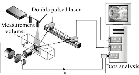
Fig.1 Schematic diagram of the experimental setup

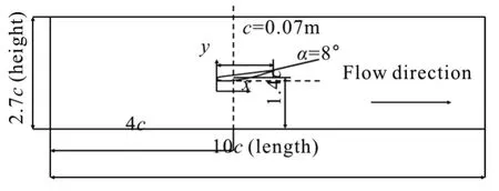
Fig.2 Sketch of the foil’s position in the test section

A two-component high-speed PIV system developed by Dantec is used, as shown in Fig.1. The light source is a dual head, Nd: YAG laser, where the beam is expanded into a 1 mm wide sheet. For the actual data acquisition, a 2000 Hz recording rate at 1024×512 pixels is chosen. The commercial PIV-soft ware,the Dynamic Studio, is applied to process the velocity vector field with an interrogation area of 32×32 pixels and 50% overlap in general. In the cavitating flows,the velocity information inside the cavity is captured using the vapor bubbles as “tracer particles”[17].

A Clark-Y hydrofoil with different angles of attack is adopted in the present study, and the chord observed at the top, bottom and sides. The cavitation tunnel is capable of generating a free stream with velocities ranging from2 m/s-15 m/s, the minimum cavitation number could be reduced to 0.3. The hydrofoil is mounted horizontally in the tunnel test section at α=0°, 5° and 8° , respectively. The foil is clamped to the back wall and the suction side of the foil is mounted toward the bottom of the test section for the convenience of viewing the cavity structures.

The data correspond to an inflow speed of 10 m/s and a cavitation number of σ=2.0. To avoid the wall boundary layer effects, the data are collected along the mid-span of the hydrofoil where the axial velocity is nearly uniform and the turbulent intensity is less than 2%. In this experimental research, the reference velocityU∞is fixed at 10 m/s, the pressure is adjusted to vary the cavitation number σ=(p∞-pv)/(0.5ρlU∞2), where p∞ is the tunnel pressure measured at the test section inlet and pv is the saturated vapor pressure, the Reynolds number isRe=U c/ν=7× 105, where ν is the kinamatic vis-∞cosity. And the Froude number iswheregis the gravitation acceleration. In general,the experimental conditions are maintained to within an uncertainty of 1% for the hydrofoil angle of incidence, and an uncertainty of 2% for both the flow velocity and the upstream pressure. The uncertainty of the electromagnetic flow meter is 0.5%, and the uncertainty of the pressure transducer is 0.25%. The cavitation number can be controlled to within an uncertainty of 5%[18,19].

2. Results and discussions

2.1 Global multiphase structures in different cavitation regimes

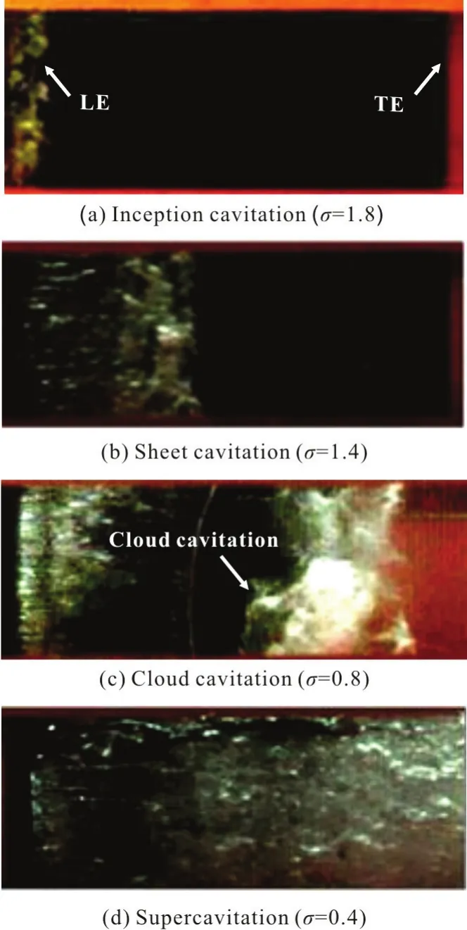
Fig.3 (Color online) Typical cavity shapes in different cavitation regimes when Re =7× 105, α=8°, viewed from the bottom of the test section

Depending on the cavitation number σ and the incidence angle α, four cavitation regimes could be identified: the inception cavitation, the sheet cavitation, the cloud cavitation, and the supercavitation.Figure 3 shows the typical cavity shapes in different cavitation regimes at σ=1.8, σ=1.4, σ=0.8 and σ=0.4 as observed in the experimental visualization, when the angle of the hydrofoil is fixed at α= 8°. Figure 4 shows the means and the fluctuations of the measured attached cavity lengths for α= 0°, α=5° and α=8° at various cavitation numbers, respectively. Cavitation inception is observed at about σ=1.8 for α=8°, which is advanced to about σ=1.6 for α=5°, and σ=1.2 for α=0°, respectively. In the regime of the inception cavitation, the cavitating flow shows in white color at the leading edge of the hydrofoil, indicating that it contains a number of micro-sized vapor bubbles.Lowering the cavitation number, the cavitation changes from the inception cavitation to a sheet cavity at about σ=1.4 for α=8°, as shown in Fig.3(b).Although the cavity is attached at the LE, the rear portion of the sheet is unsteady and it rolls up into a series of bubble eddies that shed imtermittently. The sheet cavitation begins to appear at about σ=1.3 for α= 5° and σ=1.0 for α=0°, respectively. Further decreasing the cavitation number to about σ =0.8 for α=8°, the sheet cavitation grows and the trailing edge becomes increasingly unsteady.which is accompanied with massive bubble shedding in the rear portion of the cavity, to form the cloud cavitation. In the cloud cavitation stage, the attached cavity length shows large fluctuations. It should be noted that due to the unsteady shedding of the cavity,the fluctuation amplitudes in the attached cavity are much higher for α=8° than for α=5° and α= 0°. The supercavitation is the final stage of the cavitation, At this stage, the cavitating area covers the entire hydrofoil, extending to the downstream region,the cavity boundary seems to be quite steady, as shown in Fig.3(d), and the attached cavity lengths see less fluctuations, as compared with the cases of the cloud cavitation.

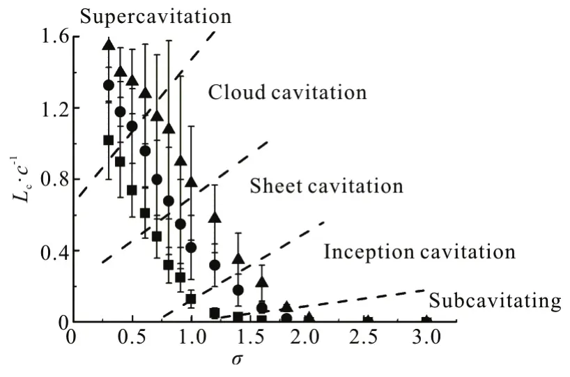
Fig.4 The measured normalized cavity lengths (L c /c) at various cavitation numbers and attack angles

2.2 The unsteady multiphase structures of cloud cavitating flows

In the cloud cavitation regime, the unsteady shedding and the breakdown occur violently, with highly unsteady hydrodynamic forces on the hydrofoil,which may lead to strong dynamic instabilities[20,21].

In the present experimental study, when the cavitation number is reduced to σ=0.4 for α=0°,σ =0.6 for α=5° and σ=0.8 for α=8°, the cavity grows and becomes increasingly unsteady until the transient cloud cavitation develops. In all above cases, it is observed that the development of the cloud cavitation assumes a distinctly quasi-periodic pattern.Figure 5 shows the side views of the periodic cavity structures, within a single flow cycle in all cases.Based on the experimental visualization, the periodsTcycleof the cloud cavitation in the case of σ=0.6 and α=5° and in the case of σ=0.8 and α=8°are almost the same, taking a value of about 40 ms,which corresponds to 5.7c/U∞, and the period in the case of σ=0.4 and α=0° is about 0.75Tcycle.

An example of a typical cavity shape observed in the experimental visualization is presented in Fig.6(a),which includes both the original flow visualization captured by the high speed camera and the schematic interpretations drawn by an in-house feature-recognition software package[22]. Figure 6(b) presents the measured time evolution of the nomarlized cavity area over several flow cycles in cloud cavitation regimes(α=0°, σ=0.4, α=5°, σ=0.6, α=8°, σ=0.8) for different attack angles. The curves see a periodic feature. The measured mean cavity areas are 0.49Sc, 0.59Scand 0.72Sc, respectively, whereScis the cross-section area of the hydrofoil.

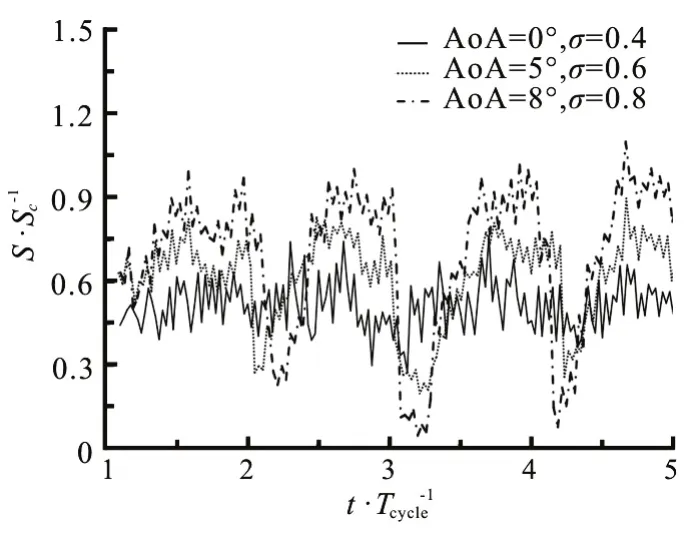
Fig.6(b) comparison of the measured time evolution of the normalized cavity area in the typical cloud cavitation regimes (α=0°, σ=0.4, α=5°, σ=0.6,α= 8°, σ=0.8), Re=7× 105, V∞ =10m/s

The void fraction distribution is of interest, and it should be related to the grayscale contours captured by the video. The mean and the standard deviation of the gray level distributions around the hydrofoil in the cases of α=0°, σ=0.4 and α=8°, σ=0.8 are shown in Fig.7, respectively. The mean cavity area is much larger in the case of σ=0.8 and α=8° than in the case of σ=0.4 and α=0°. It should be noted that the value of the standard deviation in the case of σ=0.8 and α=8° is larger than that in the case of σ=0.4 and α=0°. This is an indication of highly unsteady cavitating behavior and is typical of large-scale cloud fluctuations, as shown in Fig.5(c).

Figures 8, 9 show the evolution of the cloud shedding process in the case of σ=0.4 and α=0°and in the case of σ=0.8 and α=8°, respectively,viewed from the bottom (foil suction-side) of the test section. In the case of σ=0.8 and α=8°, the attached sheet cavity grows to its maximum length, as shown in Figs. 9(a)-9(d), and a re-entrant flow forms and pushes the flow towards the leading edge. Meanwhile, the interface becomes increasingly unsteady with the presence of bubbles due to the reverse motion of the two-phase mixture. As the re-entrant flow reaches the vicinity of the leading edge, the cavity is lifted away from the wall and shed downstream in the form of the cloud cavitation, as shown in Figs. 9(e),9(f), where the cavity shedding process is very similar to the schematic diagram of the typical cloud cavity transformation shown in Ref. [10]. The complete breakup of the cavity from the leading edge and the unsteady transformation to the cloud cavitation in the case of σ=0.8 and α=8° are different from the experimental visualization in the case of σ=0.4 and α=0°. At a smaller angle of attack, the attached cavity seems much more stable, and the cavity partially breaks at the trailing edge of the hydrofoil,followed by the successive shedding of smaller vapor structures, as shown in Fig.8.

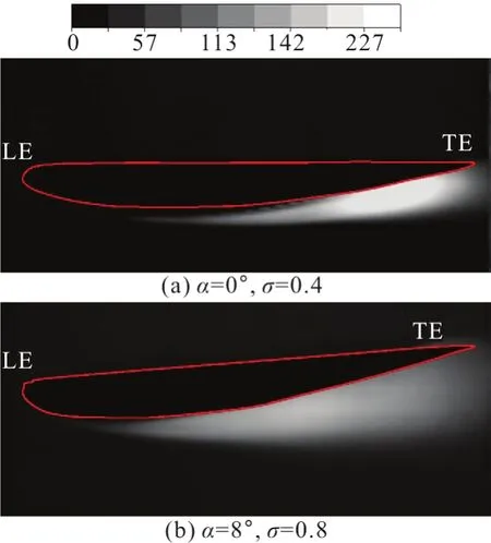
Fig.7 (Color online) Mean gray level distribution around the hydrofoil in the typical cloud cavitation regimes (α=,0°,σ=0.4, α=8°, σ=0.8), Re=7× 105, V∞=10m/s. A value of 0 corresponds to black and a value of 255 corresponds to pixel saturation (white)

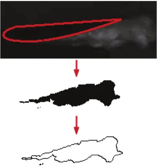
Fig.6(a) (Color online) Typical flow visualization and schematic interpretation

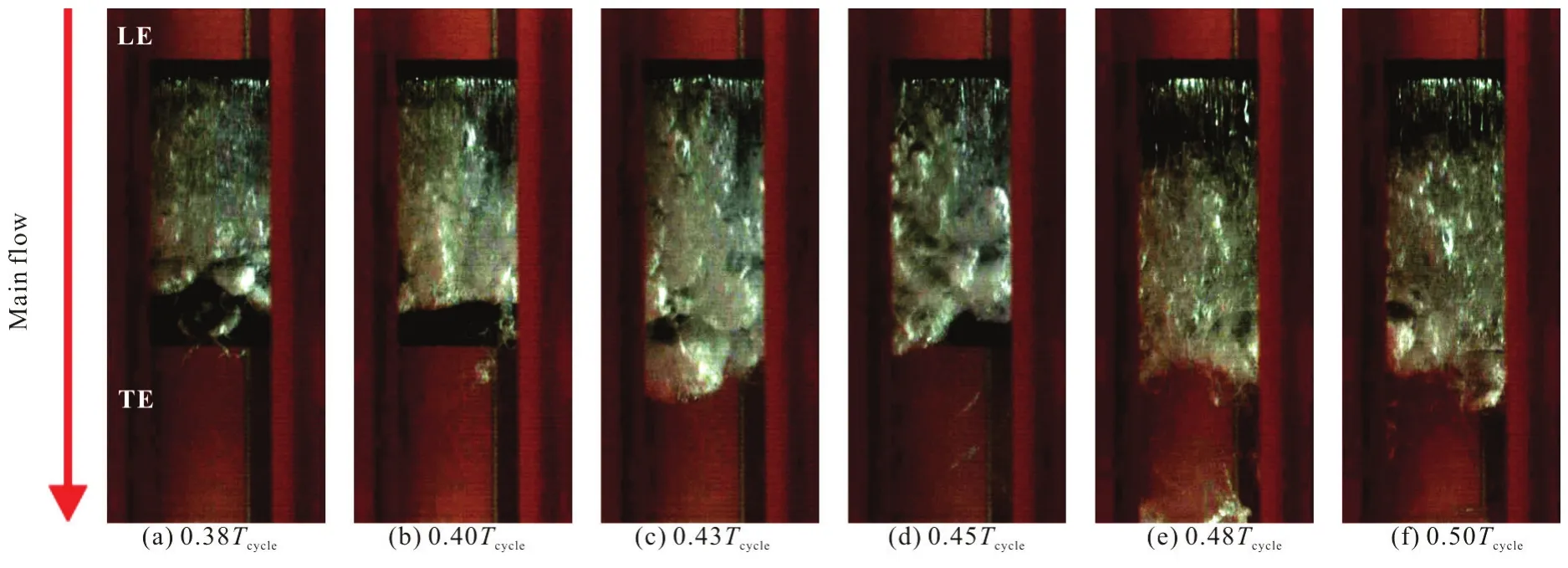
Fig.8 (Color online) Photographs of the time sequence of the cloud shedding obtained via high-speed video for σ=0.4, Re=7× 105, α=0°, viewed from the bottom (foil suction-side) of the test section

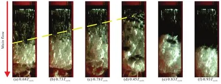
Fig.9 (Color online) Photographs of the time sequence of the cloud shedding obtained via high-speed video for σ=0.8, Re=7× 105, α=8°, viewed from the bottom (foil suction-side) of the test section

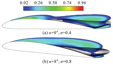
Fig.10 (Color online) Numerically predicted time-averaged cavity shapes and re-entrant flow affected regions,Re=7× 105, V=10 m/s∞

Two parameters are shown to be of the most importance in the analysis of the re-entrant flow instability: the adverse pressure gradient and the cavity thickness as compared with the re-entrant flow thickness[23]. In order to address the physical origin of the instability of the cavity at different angles of attack,Fig.10 shows the predicted time-averaged cavity shapes and the re-entrant flow affected regions in the case of σ=0.8 and α=8° and in the case of σ =0.4 and α=0° , as compared with the numerical simulation, validated with the experimental visualization and data for the same Clark-Y hydrofoil[18].Figure 11 shows the corresponding predicted contours of the negative (upstream) axial (u) velocity as a function of position and time (withTrefandLrefdefined asTref=c/U∞andLref=c). It could be concluded that the cavity thickness is directly controlled by the angle of attack, and the ratio of the thickness of the cavity to that of the re-entrant flow is substantially important to estimate the unsteady behavior of the partial cavity. In the case of σ=0.8 and α= 8°, the cavity is thick enough to limit the interaction between the re-entrant flow and the cavity interface, which allows the re-entrant flow to reach the cavity leading edge and the formation of a large scale vapor structures. However, in the case of σ=0.4 and α=0°, because of the smaller cavity thickness,one sees a strong interaction between the cavity interface and the re-entrant flow. The re-entrant flow can only reach the rear part of the hydrofoil, as shown in Fig.12, contrary to the large scale cloud shedding in the case of σ=0.8 and α=8°, where small vapor structures are formed.

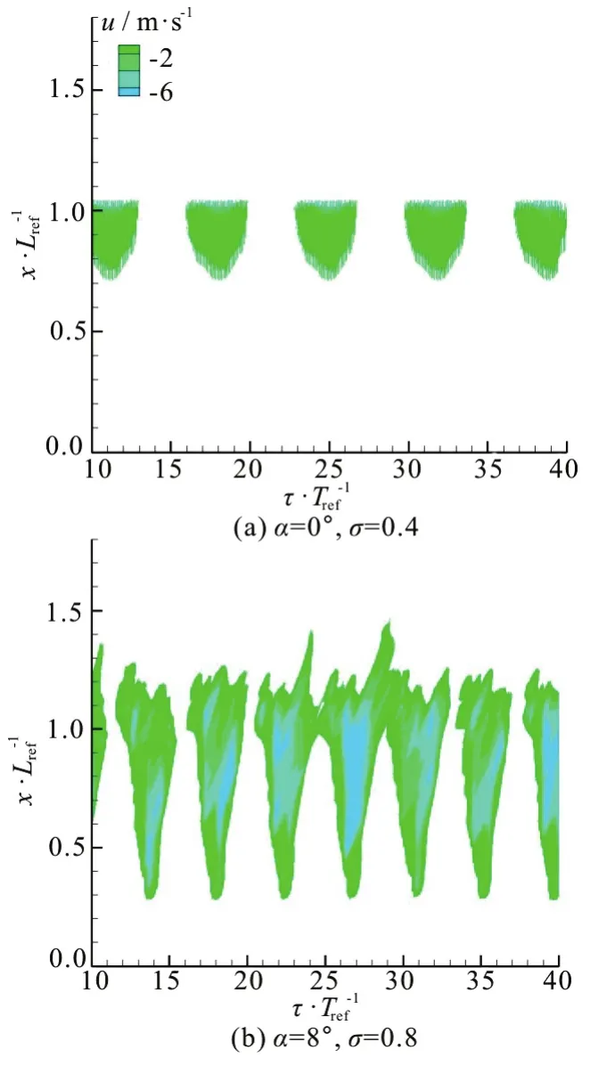
Fig.11 (Color online) Numerically predicted time evolution of the predicted reverse u-velocity in various sections (the position is in ordinate, from the foil leading edge x/ L0=0 to the trailing edge x/ L0=1), Re=7× 105,V∞=10 m/s

Fig.12 Schematic representation of the re-entrant flows in the region of an attached cavity in the typical cloud cavitation regimes (α=0°,σ=0.4,α=8°, σ=0.8)

2.3 The cavitating flow structures

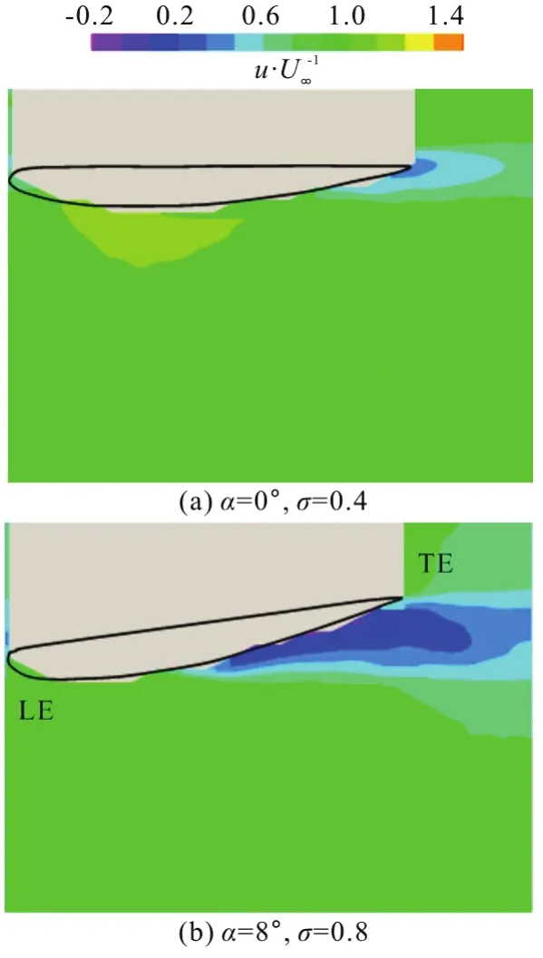
Fig.13 (Color online) Normalized ensemble averaged axial velocity contours on the suction side of the hydrofoil,Re=7×105 , V∞= 10 m/ s

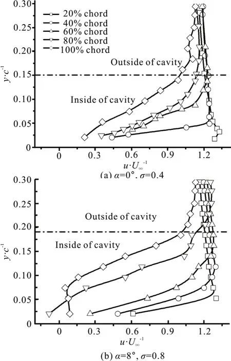
Fig.14 Means of the ensemble averaged axial velocity profiles at selected chord wise locations along the foil for cloud cavitating flow, Re=7×105 , V∞= 10 m/ s

The cavitating flow fields are measured by the PIV technology, and the images are acquired at 2000 Hz,corresponding to a mean flow displacement of 2.3% of the field of view between captures. 500 pairs of PIV images are sufficient to record more than 6 full cloud cavitation shedding cycles. Based on the measured instantaneous velocity fields, the 500 instantaneous velocity fields are averaged in the post- processing to obtain the ensemble averaged in-plane velocity and vorticity fields. Figure 13 compares the contours of the normalized ensemble averaged axial velocity which runs parallel to the inflow direction. As shown in the figure, the axial velocity near the foil trailing edge in the cavitation region is much lower. Figure 14 shows the mean values of the normalized ensemble averaged axial (u) velocity profiles at different chord wise locations in the case of σ=0.8 and α= 8° and in the case of σ=0.4 and α=0°,respectively. TheYaxis represents the vertical distance from the suction side of the hydrofoil.Substantial differences can be observed between the two cloud cavitating cases, especially near the cavity closure region. In fact, in the case of σ=0.8 and α= 8°, the recirculation breaks up and lifts the cavity upward, and the large scale shedding is formed, which significantly increases the thickness of the boundary layer and a more extended low velocity region is observed as compared to the case of σ=0.4 and α= 0°. Consequently, the gradients of the mean axial velocity profiles in the case of σ=0.4 and α=0°tend to be smaller (more evenly distributed) than those in the case of σ=0.8 and α=8°.

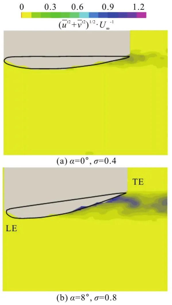
Fig.15 (Color online) Normalized amplitudes of the turbulent velocity fluctuations, Re=7× 105, V∞=10 m/s

To further investigate the turbulent velocity fields, Figure 15 shows the normalized amplitude of the averages of the fluctuating velocities,I=, in the case of σ=0.8 and α=8°and in the case of σ=0.4 and α=0°. Here,u′andv′ are the horizontal and vertical components of the turbulent velocity fluctuations. In both cloud cavitating cases shown in Fig.16, large velocity fluctuations are seen near the aft half of the hydrofoil and the fluctuation area is extended into the wake,showing the unsteady large-scale fluctuations due to the shedding of the cloud cavity, especially in the case of σ=0.8 and α=8°, meanwhile, the turbulent fluctuations are confined to a thicker layer on the suction side of the hydrofoil. Figure 17 shows the normalized amplitude of the averages of the fluctuating velocities along the selected monitor locations in the case of σ=0.8 and α=8° and in the case of σ=0.4 and α=0°. The fluctuating velocities are much higher in the case of σ=0.8 and α=8°, with a much thicker turbulent boundary layer as compared to the case of σ=0.4 and α= 0°.

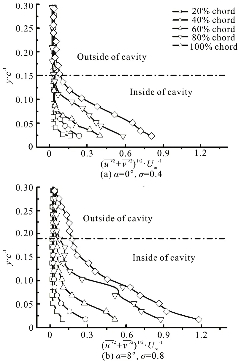
Fig.16 Normalized amplitudes of the turbulent velocity fluctuating velocity profiles at the selected monitoring locations along the foil, Re=7×105 , V∞= 10 m/ s

Figure 17 shows the side-by-side comparisons of the normalized out-of-plane (z-component) vorticity field, ωz/ωo, in the case of σ=0.8 and α=8°and in the case of σ=0.4 and α=0°. The detailed comparisons of the normalized vorticity profiles in the case of σ=0.8 and α=0° and in the case of σ =0.4 and α=0° at the selected monitoring locations are shown in Fig.18. Here, ωzis defined as:

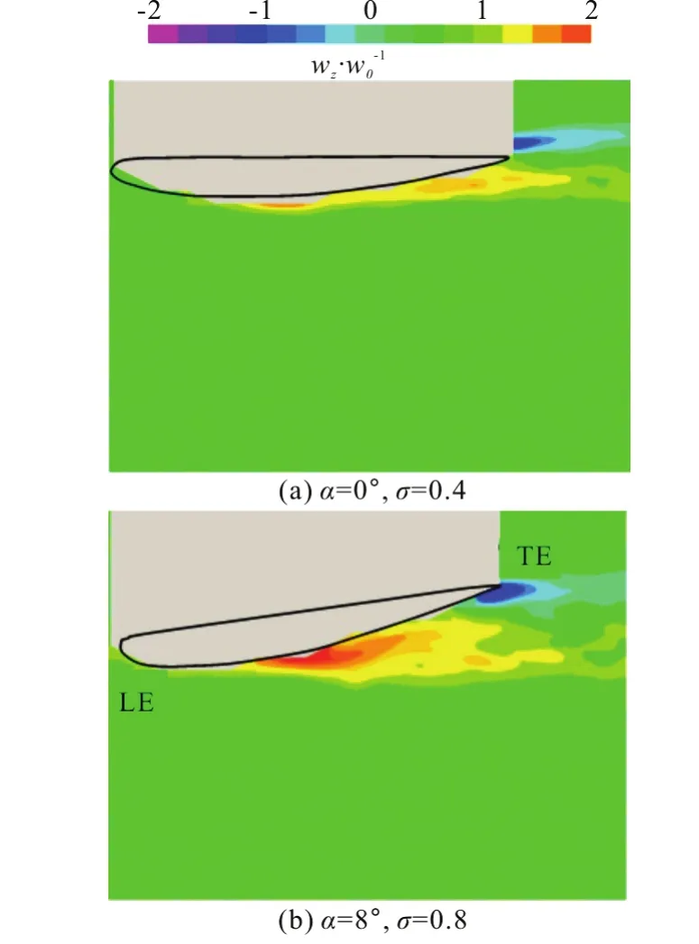
Fig.17 (Color online) Normalized averaged z -vorticity contours, ωz /ωo, on the suction side of the hydrofoil,Re=7× 105, V=10 m/s∞

( δ≈ 0.3c=0.021m is the approximated turbulent boundary layer thickness at the foil trailing edge based on the experimental measurements of the flow velocity in the cloud cavitating case of σ=0.8 and α= 8°). In both cases, large-scale counter-clockwise and clockwise vortical structures can be observed in the cavity region and at the trailing edge of the hydrofoil, respectively. Comparisons between the vorticity fields in the case of σ=0.8 and α=8° and in the case of σ=0.4 and α=0° suggest that the cavity structures play an important role in the vorticity production, in addition to the turbulent level and the turbulent boundary layer thickness. The detailed normalized vorticity profiles shown in Fig.18 in the case of σ=0.4 and α=0° suggest the existence of a thin vortical layer near the foil surface, with the thickness of the vortical zone growing toward the trailing edge, up to a maximum thickness of about 0.15c. In the case of σ=0.8 and α=8°, on the other hand, the vortical zone is much thicker (near 0.3cat the foil trailing edge), the vorticity profile is drastically different, and the magnitude of the vorticity is much larger than that in the case of σ =0.4 and α=0°.

Figure 19 shows the measured lift coefficient(CL) and drag coefficient (CD) over a range of cavitation numbers and angles of attack. When the flow is subcavitating, both lift and drag coefficients remain largely unchanged as the cavitation number varies. In the cavitation inception stage, the traveling cavity bubbles appear as shown in Fig.3, and the effect of the cavitation on the lift and drag coefficients is very small. In the subcavitating and inception cavitation stages, the hydrodynamic coefficients show little fluctuations due to the relatively stable cavity dynamics, as indicated by the error bars. Further decreasing the cavitation number, the development of the cavitation increases the drag while reduces the lift coefficient. In the cloud cavitation stage, the larger vortex shedding and the related unsteady movement strongly affect the flow structure around the hydrofoil,leading to a relatively higher magnitude of drag and a lower magnitude of lift. The combination of decreases in lift and increases in drag leads to a decrease in the efficiency, which is a classical issue for the cavitation.As indicated by the error bars of the hydrodynamic coefficients in the cloud cavitation stage, the measured values show large fluctuations, especially in the case of α=8°, which is induced by the unstable cavity dynamics. Finally, while transitioning from the cloud cavitation to the supercavitation, the cavities show more steady characteristics and both drag and lift coefficients are reduced.

2.4 Hydrodynamic coefficient

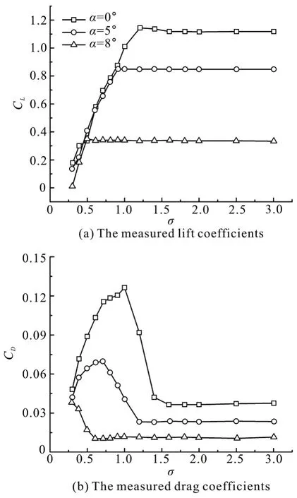
Fig.19 The measured lift coefficients and drag coefficie nts for various cavitation numbers at different angles ofattack,Re=7× 105, V=10 m/s∞

3. Conclusions

This paper investigates the unsteady structures and the hydrodynamic characteristics of the cavitating flows, to provide experimental data for future numerical validating studies. Experimental studies are for a Clark-Y hydrofoil at fixed angles of attack α=0°, 5°and 8° atRe=7× 105for various cavitation numbers,from the subcavitating flow to the supercavitation.High-speed videos of the evolution of the cloud cavitation dynamics and PIV measurements of the velocity and vorticity fields reveal the structure of unsteady cavitating flows. Statistics of the cavity lengths, the velocity distributions, the turbulent intensities, as well as the hydrodynamics are presented to better quantify the unsteady process. Detailed analysis of the cavity behavior is applied to identify the re-entrant flow instability which leads to the cloud cavitation at different angles of attack. The primary findings include:

(1) Cloud cavity is highly unsteady. High-speed photographs show a self-oscillatory behavior of the transformation from sheet to cloud cavitations. In the case of σ=0.4 and α=0°, the thickness of the attached cavity is comparable to the re-entrant flow, a relatively strong interaction is observed between the cavity interface and the re-entrant flow throughout its upstream movement. The cavity in the rear part of the hydrofoil splits into small vapor structures. In the case of σ=0.8 and α=8°, the attached cavity is thick enough to limit the interaction between the re-entrant flow and the cavity interface during its movement to the leading edge and the interface is cut, contrary to the small scale cloud shed in the case of σ=0.4 and α= 0°, the typical large vapor structures are formed.

(2) Compared to the case of σ=0.4 and α =0°, the velocities in the cavitating region are much lower, and the fluctuating velocities as well as the turbulent intensities are much higher in the cloud cavitating case of σ=0.8 and α=8°, which leads to a much thicker turbulent boundary layer. The results suggest that the periodic shedding and collapse of the vapor cavities are the important mechanisms for vorticity production, as evidenced by the production of large-scale vortical structures observed in the cavitating region of the foil and in the cavitating wake in the case of σ=0.8 and α=8°, the affected zones and the magnitude of the vorticity are much larger than those in the case of σ=0.4 and α=0°.

(3) The dynamic characteristics of the cavitation vary considerably with the angles of attack and the cavitation numbers. The effect of the inception cavity on the lift is very small, little fluctuation of the dynamic characteristics is obseved. With the decrease of the cavitation numbers, the lift is affected by the cavitating flow structure. At the cloud cavitation, the large scale shedding leads to a relatively higher magnitude of drag and a lower magnitude of lift. As the supercavitation appears, the cavity shapes and the dynamics seem more stable.

[1] Wang G. Y., Wu Q., Huang B. Dynamics of cavitation–structure interaction [J].Acta Mechanica Sinica, 2017,33(4): 685-708.

[2] Luo X. W., Ji B., Tsujimoto Y. A review of cavitation in hydraulic machinery [J].Journal of Hydrodynamics, 2016,28(3): 335-358.

[3] Wang G., Senocak I., Shyy W. et al. Dynamics of attached turbulent cavitating flows [J].Progress in Aerospace sciences, 2001, 37(6): 551-581.

[4] Peng X. X., Ji B., Cao Y. et al. Combined experimental observation and numerical simulation of the cloud cavitation with U-type flow structures on hydrofoils [J].International Journal of Multiphase Flow, 2016, 79:10-22.

[5] Franc J. P. Partial cavity instabilities and re-entrant jet [C].Fourth International Symposium on Cavitation, Paris,France, 2001.

[6] Huang B. Physical and numerical investigation of unsteady cavitating flows [D]. Doctoral Thesis, Beijing,China: Beijing Institute of Technology, 2012(in Chinese).

[7] Huang B., Ducoin A., Young Y. L. Physical and numerical investigation of cavitating flows around a pitching hydrofoil [J].Physics of Fluids, 2013, 25(10): 102109.

[8] Ji B., Luo X., Wu Y. et al. Numerical analysis of unsteady cavitating turbulent flow and shedding horse-shoe vortex structure around a twisted hydrofoil [J].International Journal of Multiphase Flow, 2013, 51: 33-43.

[9] Ji B., Luo X. W., Peng X. X. et al. Three-dimensional large eddy simulation and vorticity analysis of unsteady cavitating flow around a twisted hydrofoil [J].Journal of Hydrodynamics, 2013, 25(4): 510-519.

[10] Kawanami Y., Kato H., Yamauchi H. et al. Mechanism and control of cloud cavitation [J].Journal of Fluids Engineering, 1997, 119(4): 788-794.

[11] Fujii A., Kawakami D. T., Tsujimoto Y. et al. Effect of hydrofoil shapes on partial and transitional cavity oscillations [J].Journal of Fluids Engineering, 2007, 129(6):669-673.

[12] Kjeldsen M., Arndt R. E. A., Effertz M. Spectral characteristics of sheet/cloud cavitation [J].Journal of Fluids Engineering, 2000, 122(3): 481-487.

[13] Gopalan S., Katz J. Flow structure and modeling issues in the closure region of attached cavitation [J].Physics of fluids, 2000, 12(4): 895-911.

[14] Arndt R. E. A., Song C. C. S., Kjeldsen M. et al. Instability of partial cavitation: A numerical/experimental approach [C].Proceedings Twenty-Third Symposium on Naval Hydrodynamics, Valde Reuil, France, 2000.

[15] Ausoni P., Farhat M., Escaler X. et al. Cavitation influence on von Kármán vortex shedding and induced hydrofoil vibrations [J].Journal of Fluids Engineering, 2007,129(8): 966-973.

[16] Aeschlimann V., Barre S., Djeridi H. Velocity field analysis in an experimental cavitating mixing layer [J].Physics of Fluids, 2011, 23(5): 055105.

[17] Wosnik M., Fontecha L. G., Arndt R. E. A. Measurements in high void-fraction bubbly wakes created by ventilated supercavitation [C].ASME 2005 Fluids Engineering Division Summer Meeting, Houston, USA, 2005, 531-538.

[18] Huang B., Yong Y. L., Wang G. et al. Combined experimental and computational investigation of unsteady structure of sheet/cloud cavitation [J].Journal of Fluids Engineering, 2013, 135(7): 071301.

[19] Li X., Wang G., Zhang M. et al. Structures of super cavitating multiphase flows [J].International Journal of Thermal Sciences, 2008, 47(10): 1263-1275.

[20] Ji B., Long Y., Long X. P. et al. Large eddy simulation of turbulent attached cavitating flow with special emphasis on large scale structures of the hydrofoil wake and turbulence-cavitation interactions [J].Journal of Hydrodynamics, 2017, 29(1): 27-39.

[21] Luo X., Ji B., Peng X. X. et al. Numerical simulation of cavity shedding from a three-dimensional twisted hydrofoil and induced pressure fluctuation by large-eddy simulation [J].Journal of Fluids Engineering, 2012,134(4): 041202.

[22] Zhang M., Song X., Wang G. Design and application of cavitation flow image programs. Design and application of cavitation flow image program [C].International Symposium on Photoelectronic Detection and Imaging 2007: Image Processing, Beijing, China, 2008.

[23] Callenaere M., Franc J. P., Michel J. M. et al. The cavitation instability induced by the development of a reentrant jet [J].Journal of Fluid Mechanics, 2001, 444:223-256.