Yuan Fu (傅 渊), Da-peng Zhang (张大鹏), Xi-lin Xie (谢锡麟)

Department of Aeronautics and Astronautics, Fudan University, Shanghai 200433, China

Introduction

The rotating driven flow is a long term concern in fluid dynamics researches which is common in nature with rich phenomenon such as geostrophic current and Ekman pumping[1,2]. The systematic studies on the topic started by Greenspan[3]are of great practical value for design and development of various kinds of fluid machinery, such as turbine machine[4-6]. In the field of spin-up problem, Wells et al.[7]studied the vortices in oscillating spin-up, and the relations between spin-up and other topics have also been investigated[8-10].

In the studies of rotating system, the fluid governing equations are always written in the rotating frame of reference which is non-inertial. The advantage of it is the calculation domain can be fixed in the solving process. The time-dependent curvilinear coordinates also enjoy this feature[11-13]. Moreover, it is convenient to deal with the problems in irregular and varying physical configurations by using the time dependent curvilinear coordinates.

In the field of numerical simulation, finite difference methods in the vorticity vector-potential formulation on non-staggered grids were developed[14-16]in the past decades. Vorticity-based methods enjoy advantages not only in avoiding the calculation of pressure but also in connecting with the vorticity dynamics[17]which is an important perspective on studying flow fields. It’s also convenient to deal with Coriolis term in non-inertial frame of reference[18].

In the present study, a vorticity vector-potential method in time-dependent curvilinear coordinates is developed for two-dimensional viscous incompressible fluid in rotating system. The formula of acceleration composition in the rotating frame is derived in the curvilinear coordinates which indicates the time-dependent curvilinear coordinates is suitable for studying rotating driven flows. Tensor analysis[11,19]is adopted in deriving the component form of the governing equations. Therefore, the vorticity vector potential formulation can be discretized and solved in a regular and fixed parametric domain.

When dealing with the boundary condition of vector-potential, the rotational vector-potential of a rigid body is adopted as the vector-potential of the fluid particles on the boundary via the non-slip condition. As to the vorticity boundary condition, the conclusion is given that in two-dimensional cases the vorticity of fluid particles at the boundary intersections is twice as the rotational angular velocity of the configuration as well as the vorticity of fluid particles at the intersection lines in three-dimensional cases. The vorticity boundary condition of the rest part can be obtained by expanding the vector-potential formula in the form of contravariant components.

Thanks to the flexibility of time-dependent curvilinear coordinates in application, the method mentioned above is applied to triangle and curved triangle configurations respectively. The geostrophic effect, unsteady effect and curvature effect on the flow field evolutions are studied. Numerical results are presented for two-dimensional rotating driven flows.Moreover, the relationship between boundary vorticity,vorticity flux and the evolution process is preliminarily discussed.

1. Governing equations

1.1 Frame of reference and time-dependent curvilinear coordinates

Time-dependent curvilinear coordinates can be introduced in a rotating system, one can set (i1,i2,i3)and (e1(t) ,e2(t) ,e3(t)) as bases of inertial frame of reference and rotating frame of reference respectively.Then the rotation of the non-inertial one can be expressed as (e1,e2,e3)(t)=(i1,i2,i3)Q(t), whereQ(t) is an orthogonal matrix. The position vector of a fluid particle in flow field can be expressed in both frames of reference asr=iX(t)=e(t)Y(t). The coordinatesY(t) in non-inertial frame can be expressed in the time-dependent curvilinear coordinates as

wherex=x(ξ,t).xis the Eulerian coordinate, andξis the Lagrangian one.

In the time-dependent curvilinear coordinates,the velocityVof a fluid particle in physical domain and the material derivative of a tensor fieldΦcan be respectively expressed as:

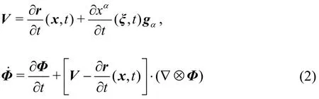
wherer=xαgα.gαdenotes the covariant base vector of the curvilinear coordinates. Einstein summation convention is employed hereinafter.

The velocity of a fluid particle can be decomposed into transport velocity and relative velocity as

and the acceleration of it can be decomposed into centripetal acceleration, Coriolis acceleration and relative one

where the relative acceleration can be expressed in the time-dependent curvilinear coordinates as

The symboldenotes the rate of change in rotational frame of reference.

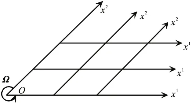
Fig.1 Sketch of calculation of particle vorticity at vertex in a two-dimensional case

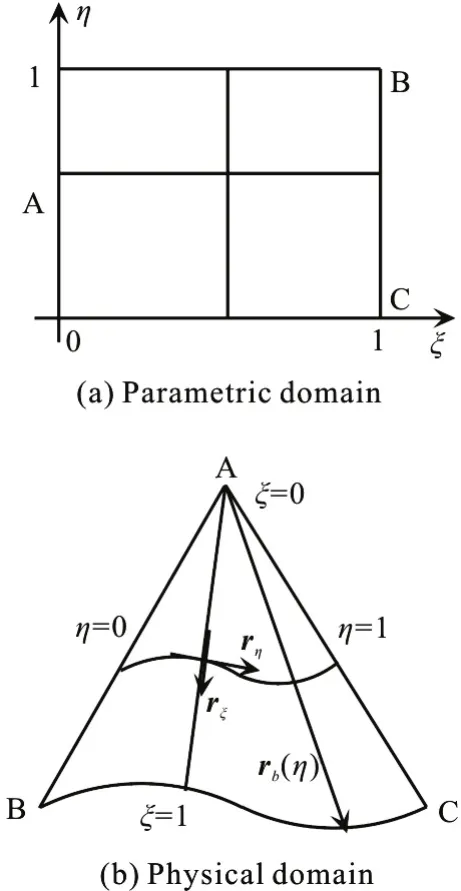
Fig.2 Sketch of a curved triangle configuration

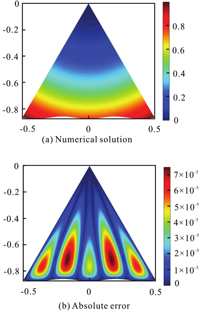
Fig.3 (Color online) Sketch of the distributions in the test of the Poisson equation solver

1.2 Vorticity vector-potential formulation

The governing equation of vorticity in inertial frame of reference can be expressed in the time dependent curvilinear coordinates as

where θ=V⋅∇ is the dilatation[20]. Meanwhile, in the rotating frame with the angular velocityΩ, the governing equation of vorticity reads

whereωris the relative vorticity in the rotating frame of reference. If the curvilinear coordinates do not include timetexplicitly, the termwill vanish, which agrees with the governing equation in Friedlander’s book. For incompressible Newtonian fluid, dimensionless governing equation of vorticity in the inertial frame of reference reads

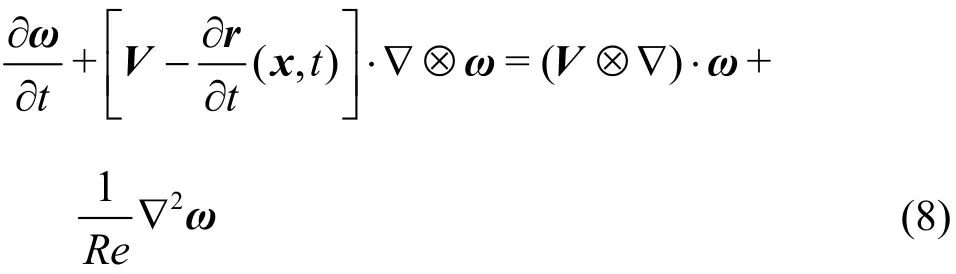
where ∂r/∂t(x,t) is also caused by the time included in the curvilinear coordinates.

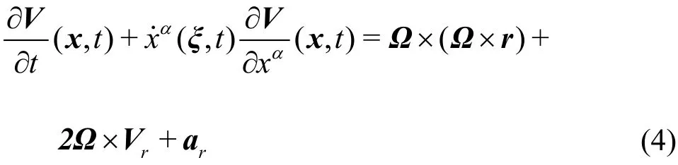
The vorticity of a fluid particle at vertex can be determined by the rotational angular velocity of the configuration. In a two-dimensional rotating system,the vorticity of a fluid particle at the boundary intersection, namely at the vertex, is twice of the rotational angular velocity of the configuration, as shown in Fig.1.

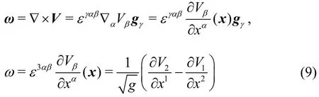
The calculation shows that the vorticity of a fluid particle at the vertex is only determined by the quantities of adjacent particles at the coordinate lines,namelyx1-line andx2-line, which are both on boundaries. Therefore the quantities ∂V1/∂x2and∂V/∂x1at vertex O are determined by the motion of 2 the configuration solely. The conclusion is consistent in three-dimensional cases in which the vorticity of a fluid particle at the intersection line is twice of the rotational angular velocity of the configuration.

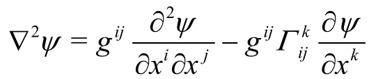
In the case of incompressible fluid, the vector potentialψcan be defined through the relationV=∇×ψ. Then the vorticity readsω=∇×(∇ ×ψ)= -∇2ψ+ ∇(∇ ⋅ψ). Under the divergence free assumption for the vector potential ∇⋅ψ=0, the governing equation of the vector-potential is ∇2ψ=-ω. For two-dimensional fluid, the stream-function ψ is the degeneration of the vector-potential and the vorticity turns intoω=ωk. Here ω is a scalar function andkis the unit vector perpendicular to the configuration plane. The governing equations turn into

2. Configuration description and boundary conditions

2.1 Configuration description in curvilinear coordinates

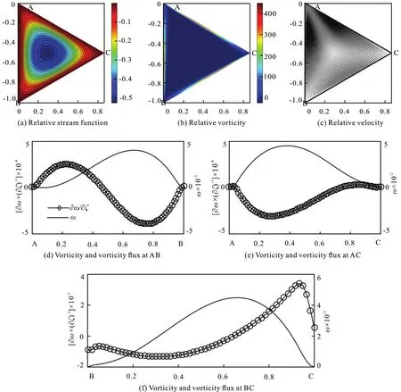
Fig.4 (Color online) Re =1000, Ω=10, t=0.05

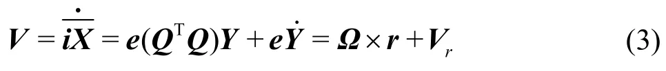
In a curved triangle, denoted by △ABC, the vertex A is set as the origin of the coordinates, and(ξ ,)η is set as the parametric coordinates. ξ=0 represents the vertex A, and ξ=1, η=0, η=1 represent sides BC, AB and AC respectively, as shown in Fig.2. A flat triangle configuration can be regarded as a special case of it.

The position vector of a point P in the curved triangle configuration can be expressed as

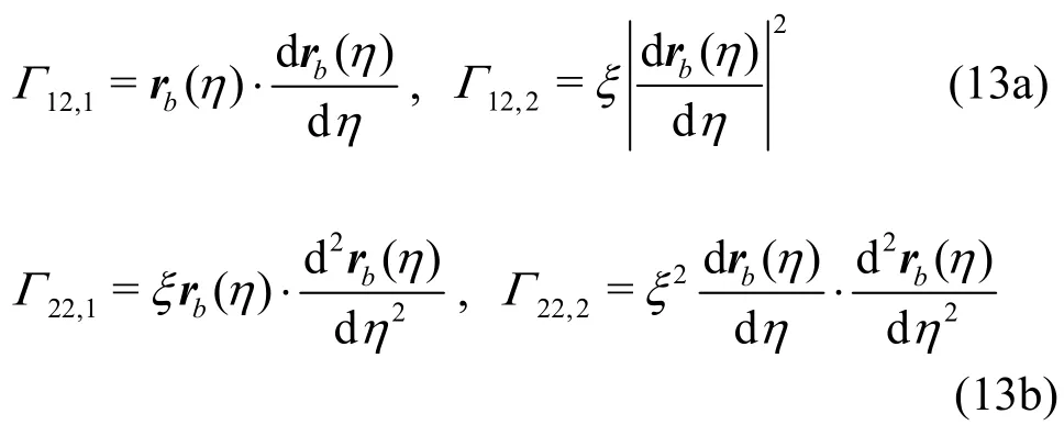
whererb(η) is a vector from the vertex A to side BC through the point P. The vector valued mappingr( ξ ,η) establishes a diffeomorphism between the parametric domainDξηand the interior of the configuration ΔABC. The covariant basis vectors of the coordinates (ξ ,)η can be calculated as

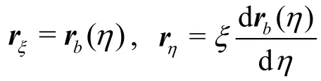
and the covariant components of the metric tensor are

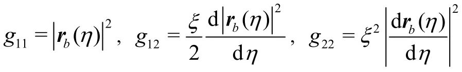
The determinant of metric matrix is

Fig.5 (Color online) Re =1000, Ω=10, t=0.79

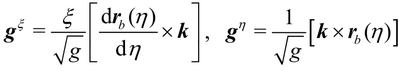
The contravariant basis vectors of the coordinates(ξ ,)η are

The non-zero second kind of Christoffel symbols can be calculated as:

and the non-zero first kind of Christoffel symbols can be calculated as:

In the case of flat triangle configurations, we have

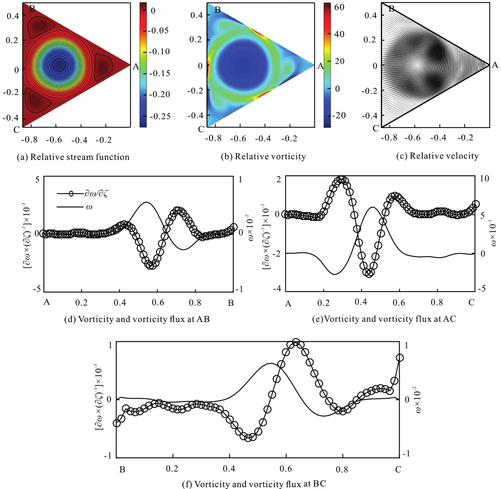
Fig.6 (Color online) Re =1000, Ω=10, t=2.36

While in the case of curved triangle configurations,the curve of BC boundary is set as

which is determined by two parameters λ and μ.Here λ determines the amplitude of the bend and μ determines the wave number of it. sinμ is forced to be zero, namely μ=kπ, in order to keep the end of vectorrCto coincide with the vertex C of BC boundary.

2.2 Boundary conditions of vector-potential and vorticity

Fig.7 Sketch of the velocity distribution of clockwise circulation in the flow field

The velocity of a fluid particle on the boundary of the configuration equals to the velocity of the rigid boundary point. So the rotational vector-potential of the rigid body is adopted as the vector-potential of fluid particles on the boundary, namely

Fig.8 (Color online) Re =1000, Ω=10, t=19.01

In the case of two-dimensional incompressible flow,the relation between stream-function ψ and contravariant components of velocity can be expressed in the parametric coordinates (ξ ,)η as:

wheregis the determinant of the coordinates.

Due to the relation2ψ=ω-∇ , the boundary condition of vorticity can be calculated by the expansion of the stream-function

In the case of three-dimensional flow, the derivatives of the contravariant components of the vector potential can be generally expressed as:

In the case of two-dimensional flow, it turns to be

It’s also worth pointing out that the singularity at the vertex A included in the formula mentioned above can be overcome by using the result that the vorticity on the vertex is twice of the rotational angular velocity of the configuration as mentioned in Section 1.2.

3. Numerical method and validation

3.1 Numerical scheme

A finite difference method is employed to carry out the spatial discretization. To be specific, a nonisometric-interval Lagrangian five-point interpolation method is adopted. The calculation grid number is 80×60. Meanwhile, the prediction-correction method is adopted to discretize time, and the time step is set as dt=1× 10-5.

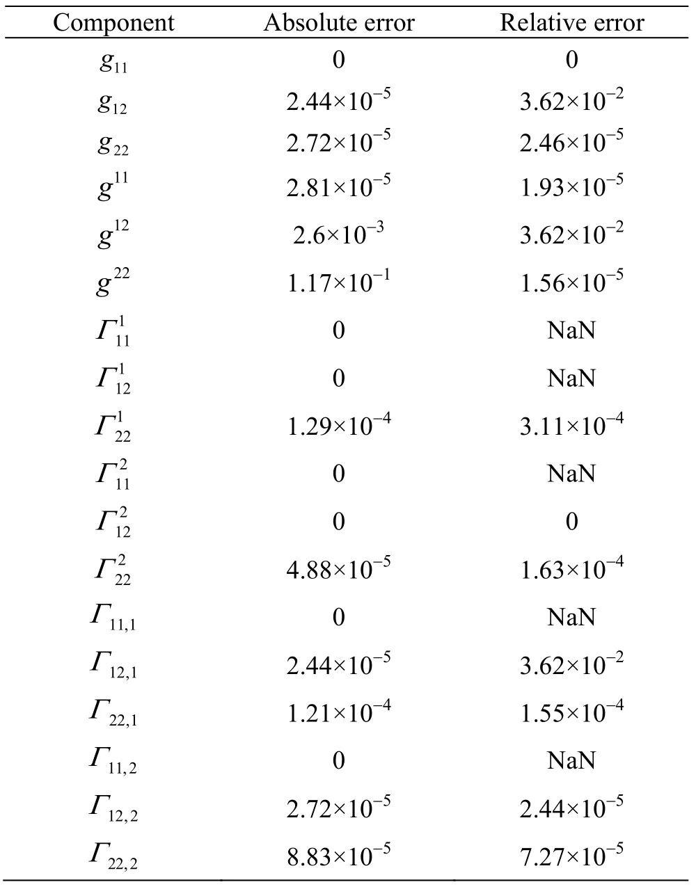
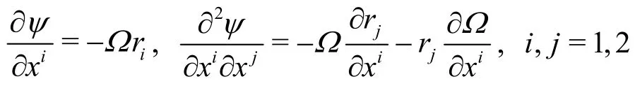
Table 1 Maximum errors of geometry quantities in the curved triangle configuration with parameters λ=0.01, μ=5π

In the test of grid quality, the geometry quantities including components of metric tensor and two kinds of Christoffel symbols are numerically calculated. The results are compared with analytical solutions. In the case of curved triangle configuration with parameters λ= 0.01, μ=5π, the numerical errors are reported in the Table 1. The symbol “NaN” implies a zero solution of the geometry quantity. The data in the table shows that the magnitude of relative errors on the whole domain is no larger than 10-4, except the data 3.6% caused by the almost-zero analytical solutions. It indicates that the grid mentioned above is acceptable.

Fig.9 (Color online) Re =1000, Ω=1, t=100.22

3.2 Validation of the Poisson equation solver

The governing equation of the stream-function is a scalar Poisson equation ∂2ψ / ∂x2+ ∂2ψ / ∂y2+f(x,y) =0. To test the solver, the source term is set asf(x,y)=-4 . The function ψ(x,y)=x2+y2is supposed to be the exact solution of the Poisson equation and the boundary condition is given correspondingly.Then the Poisson equation is mapped to the parametric domain to iterate for a numerical solution. The distributions of the numerical solution and absolute error in the curved triangle configuration are shown in Fig.3.

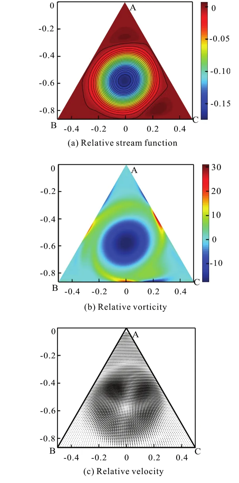
Fig.10 (Color online) Re =2000, Ω=10, t=10.05

The result shows that the maximum value of absolute error on the whole domain is 7.58×10-5, and the maximum value of relative error is 4.70×10-4. It also indicates that the numerical method mentioned above is suitable for accurately simulating the rotating system.

4. Numerical results and discussion

4.1 Constant angular velocity cases with flat boundary

In cases where angular velocity is constant, the flow field evolution can be divided into several stages.Take the case of angular velocity Ω=10,Re=1000 as an example, where the characteristic lengthLinRe=ρUL/μ is set as the length of the triangle side. At the beginning, high vorticity is generated in the middle of the boundaries by a sudden start of the configuration rotation, as shown in Fig.4.

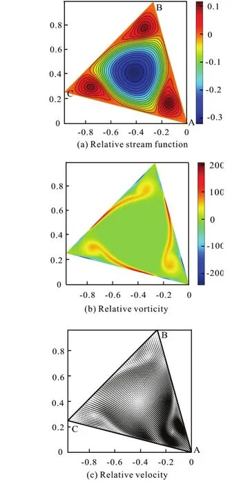
Fig.11 (Color online) Re =1000, Ω=5.5+4.5sin(5.5t),t=0.45

In the graphs here and after, thex-axis measures the scaling length of the boundary, they- axis on the left and right measure the corresponding vorticity flux and vorticity respectively, where the vorticity flux ∂/ω∂ς on the boundary represents the intensity of vorticity transportation. ς is the coordinate in direction ofnwhich is perpendicular to the boundary in configuration plane. When the boundary vorticity has the same sign as vorticity flux, the vorticity is enhancing, and vice versa.

Fig.12 (Color online) Re =1000, Ω=5.5+4.5sin(5.5t),t=0.99

At the sudden start, the vorticity at vertex B and C isas mentioned in Section1.2.The vorticity at the boundary AB and AC is positive, as shown in Fig.4. According to the Rolle theorem,the vorticity has a maximum value at the BC boundary. Actually, it reaches the peak value at the middle point of BC due to the symmetry. Considering the stress tensor at the boundary,t=-pI+2μD, whereDis the rate of strain tensor, the stresst⋅n=-pn+μω×nacts on BC. The shear stress μωis a resistance against configuration rotation. The reactive force of it is against the clockwise circulation, which is dominated by the geostrophic effect. In this case the geostrophic effect is stronger than the effect of shear stress.

Att=0.79, one end of the region where vorticity is concentrated departs from the boundary to the interior of the flow field. A clockwise circulation is formed in the middle of it, while three small counter-clockwise circulations are formed in the corner regions, as shown in Fig.5. There is an opposite tendency between the distributions of vorticity and vorticity flux at the boundary AB and AC. At boundary BC, there is an about π/2 phase difference between them.

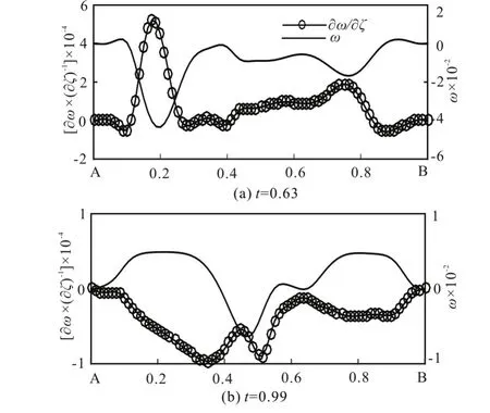
Fig.13 Re =1000, Ω=5.5+4.5sin(5.5t), vorticity and vorticity flux at boundary AB

Then, the regions of vorticity concentration are connected with each other to form a loop. The flow field is dominated by the single clockwise circulation,as shown in Fig.6. Compared with the distribution of boundary vorticity at the momentt=0.79, the vorticity flux at boundary reduces it by transporting it to inside the flow field. The amplitude of both boundary vorticity and vorticity flux decreases.

The dimensionless momentum equation in the rotating frame of reference reads

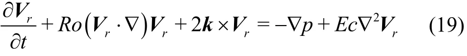
whereRo=U/ΩLandEc= ν/ΩL2denote Rossby number and Ekman number respectively.When the Rossby number is small, the convective term can be omitted. The following equation indicates the geostrophic equilibrium

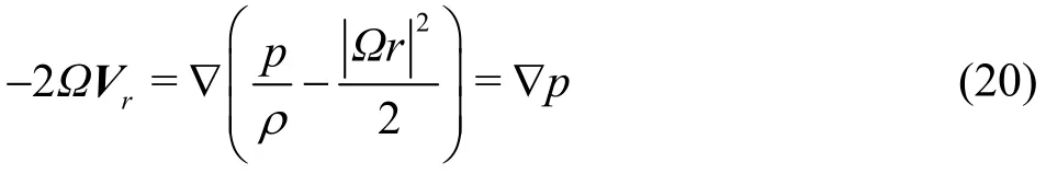
The quasi-geostrophic clockwise flow in the middle of the flow field indicates that the ∇ppoints to the center of it, as shown in Fig.7, whererCis a vector from the vertex A to the triangle center, anderis the normalization of the position vectorrwhich also starts from the vertex A.

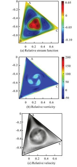
Fig.14 (Color online) Re =1000, Ω=5.5+4.5sin(5.5t),t =1.20,

Whenthere is. The result isp(rC)＞p(r). On the other hand, when, there isp(r) -p(rC). The result is alsop(rC)＞p(r). In conclusion,p(rC) is the maximum value ofpin the flow field. The direction of the circulation agrees with the result of geostrophic balance.

Att=19.01, the loop of vorticity concentration begins to dissipate.The value of vorticity flux at the boundaries is near to zero. However, the non-zero vorticity is maintained at the boundaries, as shown in Fig.8. In the process of the flow field evolution, the vorticity flux always suppresses the boundary vorticity. Then the boundary vorticity is reduced continually while the vorticity flux is near to zero on AB and AC boundaries. The vorticity flux at BC boundary is maintained a symmetric distribution and the state of flow field approaches to a geostrophic equilibrium.

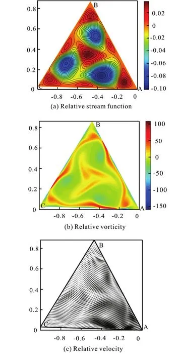
Fig.15 (Color online) Re =1000, Ω=5.5+4.5sin(5.5t),t=1.62

In the cases of constant rotational angular velocity of configuration, such as (Re=1000, Ω=1),(Re=2000, Ω=1), and (Re=2000, Ω=10), the flow field evolution goes through similar stages.. The dominated circulation in flow field is always in the opposite direction of the configuration rotation, and the amplitude of boundary vorticity and vorticity flux decreases in the evolution process. Especially, in case of (Re=1000, Ω=1), the final state of flow field is like the rotation of a rigid body. The concentration of vorticity vanishes, and the amplitude of the relative velocity drops to zero almost everywhere in the flow field, as shown in Fig.9.

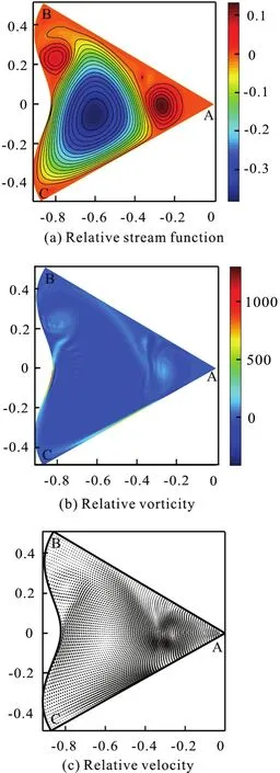
Fig.16 (Color online) μ=3π, λ=0.05, Re =2000,Ω =10, t=0.47

With a larger Reynolds number, there appears a centrifugal effect in the flow field, so that the flow pattern is slightly twisted. As shown in Fig.10, in the case of (Re=2000, Ω=10), the region of high vorticity value concentration in the middle of the flow field has an elliptical outline rather than a circular one.

4.2 Varying angular velocity cases with flat boundary

In a rotating system, rich phenomena can be created by the unsteady effect. In the case ofRe=1000,Ω =5.5+4.5sin(5.5t), the evolution process of the flow field is described as follows.

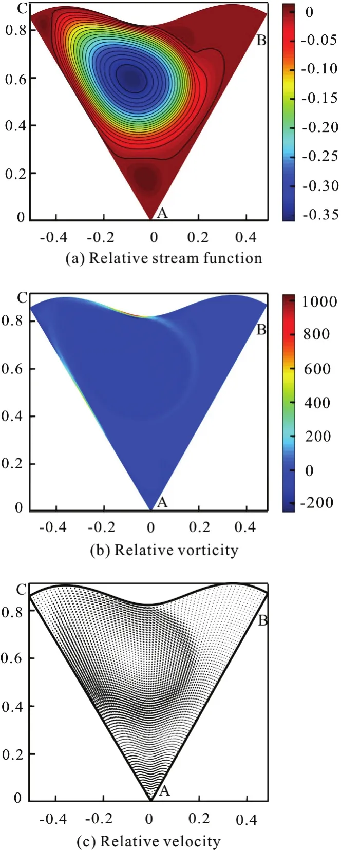
Fig.17 (Color online) μ=3π, λ=0.05, Re =2000,Ω =10, t=17.28

Firstly, as in the case of constant rotational angular velocity of configuration, the high vorticity value is generated in the middle of the boundaries and enters the flow field. A clockwise circulation is formed in the middle of the flow field and three small counter-clockwise circulations are formed at the corners, as shown in Fig.11. Due to the unsteady effect, with the decrease of the rotational angular velocity of the configuration, the counter-clockwise circulations are enhanced to dominant the whole flow field rather than vanish in the evolution. Then the counter-clockwise circulations touch each other and begin to merge.

Att=0.99, the counter-clockwise circulations merge in the middle of the flow field. A unified counter-clockwise circulation is formed, as shown in Fig.12, which is not found in the constant rotational angular velocity cases. The unsteady effect could change the flow field significantly.

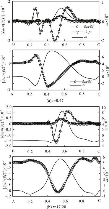
Fig.18 μ=3π , λ=0.05, Re =2000, Ω=10, vorticity and vorticity flux at boundary BC and AC

At boundary AB, there is an opposite tendency between the distributions of boundary vorticity and vorticity flux. Fromt=0.63 tot=0.99, the position of the peak value moves from 0.2 to 0.5 with the motion of the counter-clockwise circulations, as shown in Fig.13. In this process, the amplitudes of both the boundary vorticity and vorticity flux decrease.The counter-clockwise circulations move from the corner regions to the middle of the flow field.

With the increase of the rotational angular velocity of the configuration, the new clockwise circulations are formed and enhanced in the corner regions. Att=1.20, there is a counter-clockwise circulation in the interior region of the flow field and a clockwise one in the outer region of it, as shown in Fig.14.

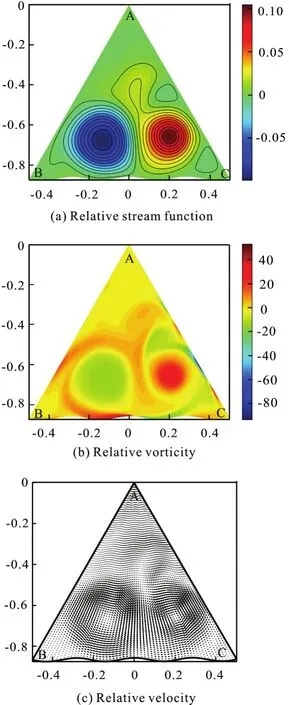
Fig.19 (Color on line) μ=7π, λ= 0.01, Re =2000,Ω =10,t=11.31

The acceleration of a fluid particle is

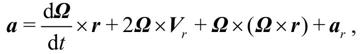
where the term

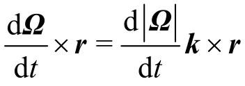
represents the unsteady effect. In the case of constant angular velocity rotation, the direction of the dominated circulation in the flow field is always clockwise which is opposite to the configuration rotation, and the geostrophic balance equation is expressed as Eq. (20). In the varying rotational angular velocity cases, the equation turns to

Fig.20 (Color online) μ=7π, λ=0.01, Re =2000,Ω =10, t=24.50

With the increase of the rotational angular velocity of the configuration, namelythe clockwise circulation is enhanced, and with the decrease of it, namelythe counter-clockwise one is enhanced instead.

With the periodic change of the rotational angular velocity of the configuration, the multi-vortex structure appears in the flow field as shown in Fig.15.Att=1.62, the flow field is dominated by three clockwise circulations, and there are small counterclockwise circulations near the boundary at the same time. The flow field evolution is quasi-periodic. Att=2 .55 there is a clock wise circulation in the flow field which is similar to the initial state of the flow field.

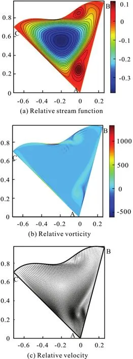
Fig.21 (Color online) μ=3π, λ=0.05, Re =2000,Ω=5.5+4.5sin(5.5t), t=0.39

In the cases of varying rotational angular velocity with flat boundary, such as (Re=1000,Ω=15+5sin(15t)), (Re=2000,Ω =5.5+4.5sin(5.5t)), and(Re=2000, Ω=15+5sin(15t)), the flow field evolution goes through similar stages as discussed above.

4.3 Constant angular velocity cases with curved boundary

Besides the unsteady effect, the curvature effect on the flow field evolution can not be omitted. In the case ofRe=2000, Ω=10 with BC boundary parameters μ=3π, λ=0.05, the evolution process of the flow field is described as follows.

In the initial stage, the dominated clockwise circulation is formed in the flow field. Meanwhile there is a small counter-clockwise circulation on the BC boundary as in backward-facing step flow. The counter-clockwise circulation enhances the dominated one. Moreover, the dominated clockwise circulation enhances another counter-clockwise circulation in the region of corner A, as shown in Fig.16.

Then the small counter-clockwise circulations slowly vanish, and the dominated clockwise circulation is fixed on the bend of BC, rotating with the configuration, as shown in Fig.17. Compared with the dominated circulations in the flat boundary configurations, the dominated one in this case shares the same direction with them which is determined by the geostrophic equilibrium. The curvature effect merely changes the position of it in this case.

There is an about π/2 phase difference between vorticity and vorticity flux on boundary BC. Att=0.47, there is an opposite tendency between the distributions of vorticity and vorticity flux at the boundary AC. The peak values of them appear at about 0.4 position, where the clockwise circulation touches the boundary. Att=17.28, the peak value position moves to 0.5, both vorticity and vorticity flux are decreased, as shown in Fig.18. In the case ofRe=2000, Ω=10 with boundary parameters μ=5π, λ=0.02, the flow field evolution goes through a similar process. The dominated clockwise circulation is fixed on the bend of BC eventually.

However, in the case of curved boundary with parameters μ=7π, λ=0.01, the flow field evolution is changed significantly by the curvature effect.After the formation of clockwise circulation in the middle of the flow field, the counter-clockwise circulation at region of corner C is enhanced rather than suppressed.

Att=11.31, there are two counter-rotating circulations in the flow field. They are both at the bends of boundary BC, as shown in Fig.19, which is not seen in other cases with the same Reynolds number and rotational angular velocity of configuration.

Eventually the counter-clockwise circulation slowly vanishes, as shown in Fig.20. The final state of the flow field is still a geostrophic equilibrium.However, the size of the clockwise circulation in this case is smaller than in others as the result of curvature effect.

4.4 Varying angular velocity cases with curved boundary

Unsteady effect and curvature effect work together in the following case. The parameters of it areRe=2000, Ω=5.5+4.5sin(5.5t), and the parameters of BC boundary are μ=3π, λ=0.05.

At the initial phase, the dominated clockwise circulation is formed in the middle of the flow field.Two small counter-clockwise circulations are formed on the BC boundary and in the region of corner A respectively, as shown in Fig.21. With the decrease of the rotational angular velocity of the configuration,the counter-clockwise circulations are enhanced due to the unsteady effect.

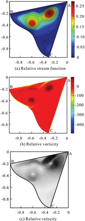
Fig.22 (Color online) μ=3π, λ=0.05, Re =2000,Ω=5.5+4.5sin(5.5t), t=0.78

In the process of the counter-clockwise circulations enhancing, they are gathered close to each other along the boundary AB, as shown in Fig.22. The curvature effect breaks the rotational symmetry of the motion path. Att=0.99, the counter-clockwise circulations merge in the middle of the flow field. A unified counter-clockwise circulation with new clockwise circulations are formed. With the increase of the rotational angular velocity of the configuration,the clockwise circulations are enhanced. Fromt=0.99 tot=1.35, the rotational angular velocity of the configuration keeps increasing, the clockwise circulations are enhanced due to the unsteady effect.Eventually a unified clockwise circulation is formed in the flow field.

The vorticity flux at the curved boundary BC can be decomposed into

here ς is the coordinate in direction ofn,Vη is the component of velocity in direction ofτ, which is the unit tangent vector of BC, and ληis the curvature of it. The distributions of these terms at different moments are shown in Fig.23. The term-ληω contains the curvature effect at the boundary BC, which vanishes in case of flat boundary configuration. Around every peak value of vorticity flux,curvature term plays an important role in the composition of it. There is an about π/2 phase difference between the boundary vorticity and vorticity flux. Fromt=0.39 tot=0.78, with the decrease of the rotational angular velocity of the configuration, the amplitudes of both vorticity and vorticity flux on BC decrease, and vice versa fromt=0.99 tot=1.35.

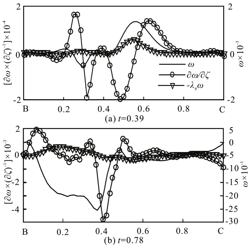
Fig.23 μ=3π,λ= 0.05, Re =2000, Ω =5.5+4.5sin(5.5t), vorticity and vorticity flux at boundary BC

In this periodic process, the increase and decrease of the rotational angular velocity of the configuration cause the enhancing of clockwise circulations and counter-clockwise ones respectively. The flow field evolution is quasi-periodic.

5. Conclusions

In this study, a numerical method based on vorticity vector-potential formulation is developed in the time-dependent curvilinear coordinates. The composition formulas of velocity and acceleration in rotating frame of reference are included in the curvilinear coordinates description. The centripetal acceleration, Coriolis acceleration and relative one can be simply expressed as two terms in this coordinates.The parametric domain is fixed and regular in the calculation process. The method is applied to the simulations of two-dimensional viscous incompressible rotating driven flows in closed configurations by overcoming the singularity at rotation axis.The numerical results in triangle and curved triangle configurations are presented by demonstrating the distributions of relative stream-function, relative vorticity and relative velocity. The flow field evolutions are discussed and classified by the shape of the configurations as well as the rotational angular velocity of them.

In the case of constant rotational angular velocity,high value of vorticity appears at the boundaries due to the sudden start of rotation. The dominated circulation which is determined by the geostrophic effect in the flow field is always in opposite direction of the configuration rotation. At AB and AC boundaries, there is an opposite tendency between the distributions of vorticity and vorticity flux, and an about π/2 phase difference between them at BC boundary. The flow fields approach geostrophic equilibrium in the final stage of the evolution. In the case of low angular velocity with small Reynolds number,the flow field behaves like a rotating rigid body eventually. Curvature effect plays different roles in different cases. Usually it changes flow fields on details, such as changing the position of circulations and the route of their motions. However, it can also change the evolution significantly, such as in the case of (μ=7π ,λ=0.01,Re=2000,Ω=10). The curvature effect doesn’t influence the direction of the dominated circulation in a flow field.

In the case of varying rotational angular velocity of the configuration, the evolution is quasi-periodic because of the periodic change of rotational angular velocity. When the rotational angular velocity of the configuration increases, the clockwise circulations in the flow field are enhanced and vice versa. The unsteady effect changes the direction of the dominated circulation from time to time, and the flow field is much more complicated than in case of constant rotational angular velocity. However, no matter how complex the evolution is, the pattern of it varies cyclically, and the pattern similar to the initial state can always be found.

The proposed method can be extended to three-dimensional situations with even more complicated configurations. It will be useful to calculate flow fields in different containers such as engines or rotating pumps. The extensions will be considered in further researches.

[1] Hardenberg J., McWilliams J. C., Provenzale A. et al.Vortex merging in quasi-geostrophic [J].Journal of Fluid Mechanics, 2000, 412: 331-353.

[2] Plumley M., Julien K., Marti P. et al. The effects of Ekman pumping on quasi-geostrophic Rayleigh-Benard convection [J].Journal of Fluid Mechanics, 2016, 803:51-71.

[3] Greenspan H. P. The theory of rotating fluids [M].Cambridge, UK: Cambridge University Press, 1968.

[4] You D., Wang M., Moin P. et al. Large-eddy simulation analysis of mechanisms for viscous losses in a turbomachinery tip-clearance flow [J].Journal of Fluid Mechanics,2007, 586: 177-204.

[5] Li L. J., Zhou S. J. Numerical simulation of hydrodynamic performance of blade position-variable hydraulic turbine[J].Journal of Hydrodynamics, 2017, 29(2): 314-321.

[6] Zhou P. J., Wang F. J., Yang Z. J. et al. Investigation of rotating stall for a centrifugal pump impeller using various SGS models [J].Journal of Hydrodynamics, 2017, 29(2):235-242.

[7] Wells M. G., Clercx H. J. H., Van Heijst G. J. F. Vortices in oscillating spin-up [J].Journal of Fluid Mechanics,2007, 573: 339-369.

[8] Foster M. R., Munro R. J. The linear spin-up of a stratified,rotating fluid in a square cylinder [J].Journal of Fluid Mechanics, 2012, 712: 7-40.

[9] Flor J. B., Ungarish M., Bush J. W. M. Spin-up from rest in a stratified fluid: boundary flows [J].Journal of Fluid Mechanics, 2002, 472: 51-82.

[10] Suh Y. K., Choi Y. H. Study on the spin-up of fluid in a rectangular container using Ekman pumping models [J].Journal of Fluid Mechanics, 2002, 458: 103-132.

[11] Xie X. L. Modern Tensor analysis with applications in continuum mechanics [M]. Shanghai, China: Fudan University Press, 2014(in Chinese).

[12] Xie X. L. On two kinds of differential operators on general smooth surfaces [J].Journal of Fudan University (Natural Science), 2013, 52(5): 688-711.

[13] Xie X. L., Chen Y., Shi Q. Some studies on mechanics of continuous mediums viewed as differential manifolds [J].Science China Physics, Mechanics and Astronomy, 2013,56(2): 432-456.

[14] E W., Liu J. Finite difference methods for 3D viscous incompressible flows in the vorticity vector potential formulation on non-staggered grids [J].Journal of Computational Physics, 1997, 138(1): 57-82.

[15] Meitz H. L., Fasel H. F. A compact-difference scheme for the Navier-Stokes equations in vorticity-velocity formulation [J].Journal of Computational Physics, 2000, 157(1):371-403.

[16] Olshanskii M. A., Rebholz L. G. Velocity-vorticity-heicity formulation and a solver for the Navier-Stokes equations[J].Journal of Computational Physics, 2010, 229(11):4291-4303.

[17] Wu J. Z., Ma H. Y., Zhou M. D. Vorticity and vortex dynamics [M]. Berlin, Heidelberg, Germany: Springer,2005.

[18] Luo H., Bewley T. R. On the contravariant form of the Navier-Stokes equations in time-dependent curvilinear coordinates systems [J].Journal of Computational Physics,2004, 199(1): 355-375.

[19] Dubrovin B. A., Fomenko A. T., Novikov S. P. Modern geometry-methods and applications [M]. Berlin,Heidelberg, Germany: Springr-Verlag, 2011.

[20] Chen Y., Xie X. Vorticity vector-potential method for 3D viscous incompressible flows in time-dependent curvilinear coordinates [J].Journal of Computational Physics,2016, 312: 50-81.