Weihong Fu*, Bin Nong, Xinbiao Zhou, Jun Liu, Changle Li School of Telecommunication engineering, Xidian University, Xi’an, Shaanxi, 7007, China Collaborative innovation center of information sensing and understanding, Xi’an, Shaanxi, 7007, China National Laboratory of Radar Signal Processing, Xidian University, Xi’an, Shaanxi, 7007, China

I. INTRODUCTION

The underdetermined blind source separation(UBSS) is one case of blind source separation(BSS) that the number of observed signals is less than the number of source signals[1]. In recent years, the technique of underdetermined blind separation is applied widely in speech signal processing, image processing, radar signal processing, communication systems[2-5],data mining, and biomedical science. Currently, many researches on UBSS have mainly focused on sparse component analysis (SCA)[6], which leads to the “two steps” approach[7].Therst step is to estimate the mixing matrix,and the second step is to recover the source signals. Notice that source signal may not be sparse in time domain, and in this case we assume that a linear and sparse transformation(e.g., Fourier transform, wavelet transform,etc.) can be found. The SCA can also be applied in the linearly transformed domain. In the “two step” approach, source signals recovery attracts very little attention, while many researchers investigate methods that identify the mixing matrix, such as clustering algorithm[8,9]or potential function based algorithm[10,11]. In this paper, we assume that the mixing matrix has been estimated successfully by the aforementioned algorithms, and we are concerned with the source signals recovery.

UBSS shares the same model with compressed sensing (CS) on the condition that the source signals are sparse and the mixing matrix is known[12]. In fact, before the concept of compressed sensing was put forward, one usual method to solve sparse BSS is to minimize the ℓ1-norm. Y Li[13]et al. analyzed the equivalence of the ℓ0-norm solution and theℓ1-norm solution within a probabilistic framework, and presented conditions for recoverability of source signals in literature[14]. But,Georgiev[15]et al. illustrated that the recovery in UBSS using ℓ1-norm minimization did not perform well ,even if the mixing matrix is perfectly known. After compressed sensing[16]technique came out, many sparse recovery algorithms were proposed, and some methods based on compressed sensing have been proposed to solve UBSS[17,18].

In 2009, Mohimani[19]et al. proposed a sparse recovery method based on smoothed ℓ0-norm (SL0), which can be applied to UBSS and is two or three times faster than the sparse reconstruction algorithm based on ℓ1-norm in the same precision or higher precision. And from then on, many scholars began to devote into the study of sparse signals reconstruction algorithm based on the SL0[20-23]. The SL0 and its improved algorithms have the advantages of less calculation and good robustness, but are easily affected by the degree of approximation of ℓ0-norm. To make the ℓ0-norm perform better, Vidya L[24]et al. proposed a sparse signal reconstruction algorithm based on minimum variance of radial basis function network (RASR). The algorithm firstly establishes a two-stage cascade network: the first stage fulfills the optimization of radial basis function, and the second stage is used for computing the minimum variance and outputting feedback to therst stage to accelerate the convergence. For the RASR algorithm,the computational complexity is not reduced obviously since two optimization models are built. What’s more, the improper step size may affect the convergence rate due to the adoption of gradient descent in the algorithm.Chun-hui Zhao[25]et al. introduce the articial neural network (ANN) into the model of compressed sensing reconstruction and obtain the compressed sensing reconstruction algorithm based on artificial neural network (CSANN),which enhances the fault-tolerant ability of the algorithm. However, the result is easy to fall into the area of local extreme point, since the penalty function of the CSANN algorithm cannot approximate the ℓ0-norm very well.In addition, the CSANN algorithm always needs a large number of iterations to end. In UBSS, the compressed sensing reconstruction algorithm mentioned above cannot meet the requirements of recovery precision of source signals and the computing complexity simultaneously. To solve the problem, we propose an algorithm for source recovery based on artificial neural network. The algorithm improves the precision of recovery by taking the Gaussian function as a penalty function to approximate the ℓ0-norm. A smoothed parameter is used to control the convergence speed of the network. Additionally, we manage to seek for the optimal learning factor to improve the recovery accuracy, and a gradually descent sequence of smoothed parameter is utilized to accelerate the convergence of the ANN. Numerical experiments show the proposed algorithm can recover the source signals with high precision but low computational complexity.

The paper is organized as follows. In Section 2, the model of UBSS based on the ANN is introduced. In Section 3, the proposed algorithm for source recovery in UBSS is presented. The performance of the proposed algorithm is numerically evaluated by simulation results in Section 4. Finally, conclusions are made in Section 5.

II. THE MODEL OF UNDETERMINED BLIND SOURCE SEPARATION BASED ON ANN

2.1 Problem description

In a blind source separation system, the received signal can be presented as

For brevity, equation (1) is rewritten as

The UBSS problem above can be viewed as a CS problem by regarding the source signalss, mixing matrixAand observed signalxin the UBSS as, respectively, the sparse signals,sensing matrix and measurement signals in the CS. So the sparse reconstruction algorithms in the CS can be readily applied to the signal recovery in the UBSS problem.

2.2 The model of articial neural network for UBSS

It is the unique knowledge structure and information processing principle that make articial neural network one of the main technologies of intelligent information processing,which attracts more and more scientific and technological workers’ interest[26]. ANN has many advantages on signal processing, including self-adaption, fault tolerance capability,etc.

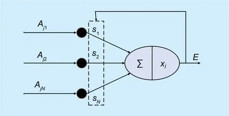
Fig. 1. The model of single-layer perceptron.

In view of the single-layer perceptron that is sufficient to describe the model of UBSS and multi-layer perceptron in which it is not easy tond optimal learning factor, we introduce the single-layer perceptron articial neural network model into UBSS in the following.As shown ingure 1,Ninputs correspond to an output. The source signal vectorsin Eq.(2)is the weight vector of the perceptron, thej-th row vectorof the mixing matrixAis the input of the perceptron model,whereis thei-th element ofAj, and thej-th elemenofxis the threshold value. The output error decision rule of the perceptron is

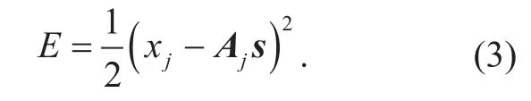
The learning procedure or the convergence process of the neural network is to minimizeEby adjusting the weight vector of the perceptron. In order to make the weight vector of the perceptron converge to the actual source signal vector, the constraint—sparsity of source signal—should be involved in the output error decision. Generally, both ℓ0-norm andℓ1-norm can measure the sparsity of source signal. To some extent, the sparse solution acquired by minimizing ℓ1-norm is equivalent to the solution obtained by minimizing ℓ0-norm in sparse recovery if mixing matrixAobeys a uniform uncertainty principle[27]. But literature[15] suggests that conditions (literature [28],theorem 7) which guarantee equivalence of ℓ0-norm and ℓ1-norm minimization are always not satisfied for UBSS. Hence, ℓ0-norm is used as a penalty function to further adjust the weight coefcients, and Eq. (3) can be rewritten as

whereγ＞0 is used to trade off the penalty function and the estimation error. For ease of analysis, we assumeγ=1. Since the minimization of the ℓ0-norm of source vectorsis an NP-hard problem, literature [25] uses Eq. (5)to approximate the ℓ0-norm.

whereβ＞0, and the greater the value ofβis, the better it is able to approximate the ℓ0-norm. CSANN algorithms generally use the empirical valueβ=10.

In Eq. (5), however, the operation of taking absolute value leads to terrible smoothness of function. In order to approximate the ℓ0-norm more perfectly, the Gaussian function is introduced as the penalty term, and Eq. (5) can be rewritten as

whereσ＞ 0, and the smallerσis, the better it is able to approximate the ℓ0-norm. Figure 2 illustrates the results of calculating the ℓ0-norm by using Eq. (5) and Eq. (6) respectively. Obviously, both Eq.(5) and Eq.(6) can reflect the characteristic of ℓ0-norm, but the result of approximating ℓ0-norm using Gaussian function is better than another. In order to further compare the degree of approximating the ℓ0-norm using the two penalty functions aforementioned, we produce a 12×20 signal matrix (12 and 20 are the number of sources and the number of sampling respectively) with sparsity (dened in Section 4) 0.75 to approximateℓ0-norm by the two functions. As shown ingure 3, the horizontal coordinate is the discrete sampling time (t=1,2,…,20), and the vertical coordinate is the value of the ℓ0-norm calculated by different functions and it demonstrates that the value of ℓ0-norm obtained by Eq. (6) is closer to the theoretical value. In addition, the average error of Eq.(6) is only0.0501, while the average error of Eq.(5) is 1.8107. Thus, it is better to use the Gaussian function to approximate the ℓ0-norm.

If the value ofσis small enough, by substituting Eq. (6) into Eq. (4) we obtain that

Fig. 2. Comparison of approximation of ℓ0-norm by different functions.

Fig. 3. The comparison between two functions f or approximating ℓ0-norm and their theoretical values.

The procedure of source recovery in the UBSS based on the ANN adjusts the weight vector of the perceptron according to the output error decisionE. Moreover, a gradient descent is used in order to increase the learning speed of the neural network and improve recovery accuracy. Then we manage to calculate the optimal step size, which we call it learning factor here.When the convergence condition is satisfied,the obtained weight vector of the perceptron is the estimated source signal vector.

III. ALGORITHM FOR SOURCE RECOVERY BASED ON ANN

Eq. (8) is used as the convergence criterion for the CSANN algorithm, that is

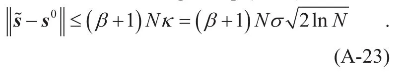
whereε＞0, ifεis small enough, the process of algorithm will get to the nearly ideal state of convergence, but more iterations are needed. According to [24], in practice, the CSANN algorithm requires the maximum number of iterations to terminate its iteration and the complexity is intolerable. In order to improve the precision of recovery, the maximum number of iterations in the CSANN algorithm will be a large value and it consumes much time. Trade-off between fewer numbers of iterations and higher accuracy of source signal recovery is a main difculty to achieve.To solve this difficulty, a gradually descent sequence of smoothed parameterσutilized in Eq.(7) is used to assure the convergence of the proposed algorithm and the accuracy of source recovery simultaneously. Explanations for the decent sequence can be found in [19]. We can prove that

wheres0is the most sparse solution of UBSS problem (i.e. Eq.(1)) ands~ is the optimal solution of Eq.(7). The process of proof is shown in appendix A.

However, the functionEin Eq.(7) is highly non-smoothed for small values ofσand contains a lot of local maxima, which leads to tough maximization. On the contrary,Eis smoother and contains less local maxima ifσis large, which results in easier maximization.But the second term of Eq. (7) cannot approximate ℓ0-norm well for largeσ.

Therefore the convergence condition is

Whereσminshould be small as small as possible but cannot be too small.

For Eq.(7), the gradient descent method is used to adjust the weight coefficients of the perceptron. Calculating the gradient vector of Eq. (7), we obtain that

Therefore, the updated formula for the weight coefcients of perceptron is

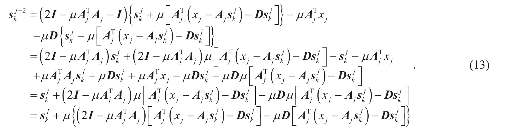
Substituting Eq. (11a) into Eq. (12) yields Eq. (13) shown in the bottom at next page.

Comparing (13) to (11a), and meanwhile due toEq.(14) can be obtained:

Then, Eq. (14) is rewritten as

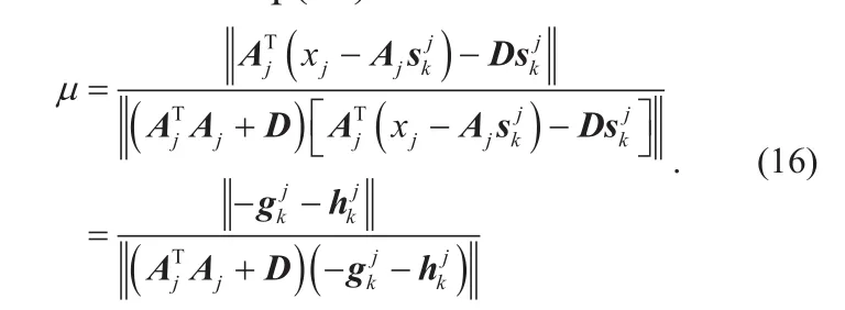
So far, the optimal learning factor can be obtained from Eq.(15)

According to the above mentioned analysis, the process source recovery for the UBSS based on the articial neural network contains only one optimization problem, which can improve the accuracy of source recovery and dramatically reduce computational cost.

In summary, the steps of the UBSSANN algorithm are as following:

Step 1Initialize the source signal vectorparameters of Gaussian functionthe scale factorδ(0＜δ＜1, used to implement decent sequence ofσ), the threshold valueσmin≤10−2and the number of iterationsk=0;

Step 2For, calculateusing Eq.(11a) and (16);

Step 3Update the smoothed parameter of Gaussian function:

Step 5Ifσk＞σmin, go to step 2; otherwise,output

Step 4Update the number of iteration:k←k+1；

The computational complexity of the SL0,CSANN and RASR algorithms has been analyzed in the literature[20]. Analysis and experimental results show that the computation time of the RASR algorithm is only half of that of the SL0, and the number of iterations in the RASR algorithm is signicantly smaller than that in the CSANN algorithm, and the convergence time of the CSANN algorithm increases exponentially with the growth of the number of non-zero elements in the source signal. For the convenience of comparison, a contrast mode in literature [20] is used. The index of measuring complexity is the number of multiplication consisting in the gradient descent method to update the source signal.

As shown in Table 1, the computational complexity of the UBSSANN algorithm is lower than that of the SL0, CSANN and RASR algorithms in the case of low degree of sparsity and high degree of sparsity. The structure and characteristics of the SL0,CSANN, RASR and UBSSANN algorithms are presented in Table 2. For the RASR, it contains two optimization models while the UBSSANN contains one optimization model,which implies that it is easier to optimize for the UBSSANN.

IV. SIMULATION RESULTS AND NUMERICAL ANALYSIS

In this section, the simulation results of the proposed UBSSANN algorithm are compared with those of the other algorithms (the SL0,CSANN, and RASR). In order to evaluate the accuracy of recovery for different algorithms,the correlation coefcient[21]is dened as:

whereSandSˆ denote the source signal and the estimated signal respectively,is then-th row andj-th column ofS,sˆn(t) denotes then-th row andj-th column ofSˆ. The larger the correlation coefcient is, the more accurate the algorithm will be. The value ofρ(Sˆ,S)ranges from 0 to 1.The sparsitypis dened as following: each source is inactive with probabilitypand is active with probability 1-p.pcontrols the degree of sparsity of the source signal. Source signal becomes sparser with increasingp.

Table I. Computational complexity of the four algorithms.

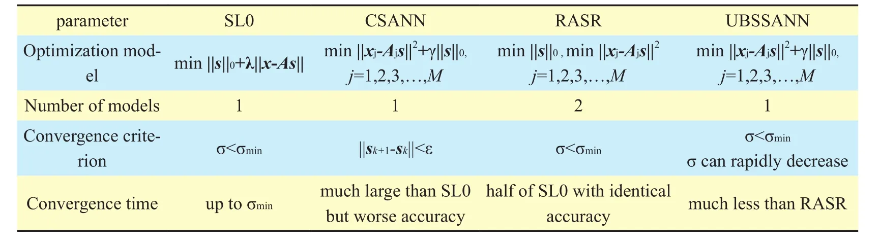
Table II. Comparison of algorithm structure feature.

Firstly, in order to analyze the effect of parameters on the algorithm performance, parameters are tested for different SNR (signalto-noise ratio) and sparsity of source signals.Secondly, according to the results in the first experiment, we choose appropriate value of parameters and compare the proposed algorithm with conventional algorithm in the second experiment for random signals. Finally,radar signals are used in the third experiment to prove the availability of the proposed UBSSANN algorithm in a real scenario.

4.1 Simulation for eect of parameters on performance

In order to verify the performance of the proposed algorithm, the effect of parameters on algorithm performance is studied in this experiment. Two essential parameters, the scale factorδand convergence threshold valueσmin,are discussed. With different sources randomly generated and a mixing matrix of dimension 8×15, the simulations are repeated 100 times.

In figure 5, the number of iterations corresponding to the scale factor is depicted for different SNRs and the sparsity of source signal. Fromgure 5(a) orgure 5(b), we can roughly conclude that the number of iterations will rapidly increase when the scale factor is greater than 0.6. Hence, in the next experiment, the scale factorσis set as 0.6 such that the convergence is accelerated.

4.2 Simulation results for random source signals

Source signals, following Gaussian distribution, are sparse signals with sparsityp∈[0.5,0.9], which are received byMantennas. The source signal becomes sparser with increasingp. A mixing matrix is of dimensionM×N, which is randomly generated with the normal distribution. Simulations are repeated 1000 times. For the SL0, RASR and UBSSANN algorithms,σminis set as 0.001.The convergence criteria of the CSANN algorithm isand the maximum number of iterations isxed to 500.

Fig. 4. Effect of parameters on performance.

Figure 6 demonstrates the correlation coefficient obtained by different algorithms corresponding to SNR for different system scales (i.e., the dimension of mixing matrix,MandN, mentioned in section 2) in the case ofp=0.8. As shown ingure 6, the correlation coefficient of the UBSSANN algorithm is obviously larger than that of all the other algorithms. For instance, the correlation coefcient obtained by the UBSSANN is about 6%, 10%,15% higher than that by the RASR,SL0 and CSANN, respectively, when SNR is 20dB in case ofM=3,N=5. This improvement on the correlation coefficient is essential for many real applications, such as radar signal processing. In the range of SNR from 10 dB to 20 dB, the average correlation coefcients of the UBSSANN algorithms are 0.9034, which shows its robustness against the noise.

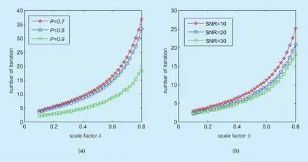
Fig. 5. The number of iterations varies with the parameter scale factor.

Figure 7 shows the correlation coefficients obtained by the SL0, CSANN, RASR,UBSSANN algorithms corresponding to sparsitypwith several mixing matrices of different dimensions in the case where SNR is 30 dB.When the sparsitypis greater than 0.6, the correlation coefficient of the UBSSANN algorithm is larger than that in the SL0, RASR,CSANN algorithms. For example, in the case ofp=0.8,M=6,N=10, the correlation coefficients obtained by the UBSSANN algorithm are about 4%, 10% and 22% larger than that of the RASR, CSANN and CSANN algorithms,respectively. As presented in Table 1 and Table 2, however, the complexity of the UBSSANN is signicantly lower than that of the conventional algorithms. When the sparsity is less than 0.6, the correlation coefficient of the UBSSANN algorithm is a little smaller than that of the RASR but larger than that of SL0 and CSANN.

Figure 8 shows the contrast between the correlation coefficients obtained by the UBSSANN and RASR corresponding to the number of iterations in the case of SNR=20dB andp=0.9 at axed time. Figure 6 illustrates that the UBSSANN algorithm has reached the convergence state in the 5th iteration, while the RASR is close to the state of convergence after the 20th iteration. So the convergence rate of the UBSSANN is relatively fast.

In the following，we give the time required by different algorithms. As shown ingure 9,in the case of SNR=20dB, the running time of UMSRANN algorithm is less than the other three algorithms. With the range of sparsity from 0.5 to 0.9, the average running time of UBSSANN algorithm is reduced by about 40%, 60% and 29% respectively compared with SL0, CSANN and RASR algorithm. It implies that UBSSANN algorithm maintains high recovery accuracy while signicantly re-duce the computational complexity compared with the other three algorithms.

Fig. 6. Correlation coef cient vs. SNR with p=0.8 for different dimension mixing matrix.

Fig. 7. Correlation coef cient vs. sparsity p with SNR=10dB for different dimension mixing matrix.

4.3. Simulation results for radar source signals

In this experiment, 5 radar signalsare chosen as the source signals.are general radar signals with the same pulse width 10µsand pulse duration 50µs,but with different carrier frequencies 5MHz and 5.5MHz.s3is linearly frequency modulated (LFM) radar signal with a carrier frequency 5MHz, pulse width 10µs, pulse duration 50µsand pulse bandwidth 10MHz.s4is also a LFM radar signal with the same parameters ass3, but its pulse bandwidth is 15MHz.s5is a sinusoidal phase-modulated radar signal with a carrier frequency 5MHz, pulse width 10µs,pulse duration 50µsand the frequency of sine-wave modulation signal 200KHz. The dimension of mixing matrix isM=3,N=5(i.e.,3 receiving antennas and 5 source signals). To assess the recovery equality, signal-to-interference ratio (SIR) of recovery source signal is used here besides the correlation coefficient,and the SIR of recovery source signal is defined aswheresanddenotes the real source signal and recovery source signal, respectively.

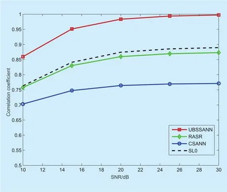
Fig. 8. correlation coef cient vs. iterations of UBSSANN and RASR algorithms respectively.

Fig. 9. computing time vs. degree of sparsity with SNR = 20 dB.

In this experiment, we use the SL0,CSANN, RASR, and UBSSANN algorithms to recover the source signals. Figure 10 and figure 11 demonstrate the correlation coefficient and SIR of the recovered signals obtained by the aforementioned algorithms,respectively. As shown in figure 10, the UBSSANN algorithm gives good results for the SNR ranging from 10 dB to 30 dB, performing better than the SL0, CSANN, and RASR in terms of correlation coefcient. For instance, correlation coefficient acquired by the UBSSANN is about 0.99, while those obtained by the SL0, RASR and CSANN are about 0.89, 0.87, 0.76, respectively, when SNR=30dB. Instead of correlation coefcient, the SNR of the recovered signal is used to evaluate the algorithms’ performance, as shown ingure 11. Obviously, the SIR of the recovered signal obtained by the UBSSANN is significantly greater than those acquired by the SL0,CSANN, and RASR while the SNR of mixed signal ranges from 10 dB to 30dB. Moreover,the SIRs obtained by the SL0, CSANN, and RASR are all lower than 10dB while that obtained by that UBSSANN roughly linearly increases with respect to the SNR of the mixed signal rising.

V. SUMMARY

For the problem of high computational complexity when the compressed sensing sparse reconstruction algorithm is used for source signal recovery in UBSS, the UBSSANN algorithm is proposed. Based on the sparse reconstruction model, a single layer perceptron articial neural network is introduced into the proposed algorithm introduces, and the optimal learning factor is calculated, which improves the precision of recovery. Additionally,a descending sequence of smoothed parameterσis used to control the convergence speed of the proposed algorithm such that the number of iterations can be signicantly reduced.Compared with the existing algorithms (i.e.,SL0, CSANN and RASR) the UBSSANN algorithm achieves good trade-off between the precision of recovery and computational complexity.

Fig. 10. Correlation coef cient vs. SNR of mixed signal.

Fig. 11. SIR of recovered signal vs. SNR of mixed signal.

Appendix A

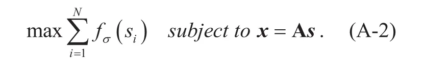
UBSSANN’s original mathematical model is

whereNrepresents the number of source sig-nals,Obviously, (A-1)is equivalent to

Then

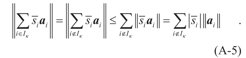
According to Eq. (A-5) and (A-6), we can get that

It is assumed that Aˆ is a sub-matrix composed ofaivectors in matrix A, wherei∈Iκ, then Aˆ contains at mostMcolumn vectors. Since each column vector is independent of each other, Aˆ has left pseudo inverse,denoted asIn addition, in the vectorthe sub-vector corresponding to the element constituting the subscript setIkis denoted byand the sub-vector of the element corresponding to the subscript which is not belong toIkis denoted ass′,

We can get that

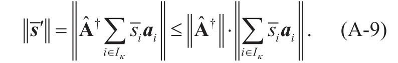
According to Eq. (A-7), it can be obtained that

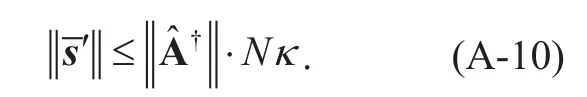
Similarly, combining with Eq.(A-6), we get

By Eq. (A-10) and (A-11), it can be obtained that

The set of all the sub-matrices Aˆ of the mixing matrix A is now referred to as Θ, Letβbe as follow:

Then

Next we use Eq. (A-14) to prove that

wheres0is the most sparse solution of UBSS problem (i.e. Eq.(1)) ands~ is the optimal solution of Eq.(7).

It is assumed that the vectorsatisfies the constraintx=As~ and is the optimal point of the current objective functionThe set of subscripts corresponding to the elements satisfyingin vectors~ is denotedthere is

Combined with Eq. (A-3), it can be obtained that

Sinces~ is the optimal point of the current objective function, then

According to Eq. (A-17), (A-18) and (A-19), we get

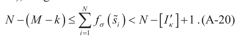
Then

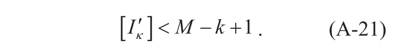
So

Therefore, the number of elements ofwhose absolute value is bigger thanκis at mostM−k, and that of non-zero elements ofs0is at mostk, so the number of elements inwhose absolute value is bigger thanκis at mostM−k+k=M.

Then

ACKNOWLEDGMENT

This work was supported by National Nature Science Foundation of China under Grant(61201134, 61401334) and Key Research and Development Program of Shaanxi (Contract

No. 2017KW-004, 2017ZDXM-GY-022).

[1] G. R. Naik, W. Wang, Blind Source Separation:Advances in Theory Algorithms and Applications (Signals and Communication Technology Series), Berlin, Germany: Springer, 2014.

[2] Gao, L., Wang, X., Xu, Y. and Zhang, Q., Spectrum trading in cognitive radio networks: A contract-theoretic modeling approach. IEEE Journal on Selected Areas in Communications, 2011，29(4), pp.843-855.

[3] Wang, X., Huang, W., Wang, S., Zhang, J. and Hu, C.,Delay and capacity tradeoanalysis for motioncast. IEEE/ACM Transactions on Networking (TON), 2011，19(5), pp.1354-1367.

[4] Gao, L., Xu, Y. and Wang, X., Map: Multiauctioneer progressive auction for dynamic spectrum access. IEEE Transactions on Mobile Computing, 2011，10(8), pp.1144-1161.

[5] Wang X, Fu L, Hu C. Multicast performance with hierarchical cooperation[J]. IEEE/ACM Transactions on Networking (TON), 2012, 20(3): 917-930.

[6] Y. Li, A. Cichocki, S. Amari, “Sparse component analysis for blind source separation with less sensors than sources”,Proc. Int. Conf. Independent Component Analysis (ICA), pp. 89-94, 2003.

[8] J. Sun, et al., “Novel mixing matrix estimation approach in underdetermined blind source separation”,Neurocomputing, vol. 173, pp. 623-632, 2016.

[9] V. G. Reju, S. N. Koh, I. Y. Soon, “An algorithm for mixing matrix estimation in instantaneous blind source separation”,Signal Process., vol. 89, no.3, pp. 1762-1773, Mar. 2009.

[10] F. M. Naini, et al., “Estimating the mixing matrix in Sparse Component Analysis (SCA) based on partial k-dimensional subspace clustering”,Neurocomputing, vol. 71, pp. 2330-2343, 2008.

[11] T. Dong, L. Yingke, and J. Yang, “An algorithm for underdetermined mixing matrix estimation”,Neurocomputing, vol. 104, pp. 26-34, 2013.

[12] T. Xu, W. Wang, “A compressed sensing approach for underdetermined blind audio source separation with sparse representation”,Proc.IEEE Statist. Signal Process. 15th Workshop, pp.493-496, 2009.

[13] Y. Q. Li, A. Cichocki, S. Amari, “Analysis of sparse representation and blind source separation”,Neural Comput., vol. 16, no. 6, pp. 1193-1234,2004.

[14] Y. Li, et. al., “Underdetermined blind source separation based on sparse representation”,IEEE Trans. Signal Process., vol. 54, no. 2, pp. 423-437, Feb. 2006.

[15] P. Georgiev, F. Theis, A. Cichocki, “Sparse component analysis and blind source separation of underdetermined mixtures”,IEEE Trans. Neural Networks, vol. 16, no. 5, pp. 992-996, Jul. 2005.

[16] D. Donoho, “Compressed sensing”,IEEE Trans.Inform. Theory, vol. 52, no. 4, pp. 1289-1306,Apr. 2006.

[17] T. Xu, W. Wang, “A block-based compressed sensing method for underdetermined blind speech separation incorporating binary mask”,Proc. Int. Conf. Acoust. Speech Signal Process.(ICASSP), pp. 2022-2025, 2010.

[18] M. Kleinsteuber, H. Shen, “Blind source separation with compressively sensed linear mixtures”,IEEE Signal Process Lett., vol. 19, no. 2, pp. 107-110, Feb. 2012.

[19] H. Mohimani, M. Babaie-Zadeh, and C. Jutten,“A Fast Approach for Overcomplete Sparse Decomposition Based on Smoothed L0 Norm”,IEEE Trans. Signal Process., vol. 57, no. 1, pp.289-301, Jan. 2009.

[20] A. Eftekhari, M. Babaie-Zadeh, C. Jutten, H.Abrishami Moghad-dam, “Robust-SL0 for stable sparse representation in noisy settings”,Proc. Int. Conf. Acoust. Speech Signal Process.(ICASSP), pp. 3433-3436, 2009.

[21] S. H. Ghalehjegh, M. Babaie-Zadeh, and C. Jutten, “Fast block-sparse decomposition based on SL0”,International Conference on Latent Variable Analysis and Signal Separation, PP. 426-433, 2010.

[22] Changzheng Ma, Tat Soon Yeo, Zhoufeng Liu.“Target imaging based on ℓ1ℓ0 norms homotopy sparse signal recovery and distributed MIMO antennas”,IEEE Transactions on Aerospace and Electronic Systems, vol.51, no.4, pp:3399-3414,2015

[23] V. Vivekanand; L. Vidya, “Compressed sensing recovery using polynomial approximated l0 minimization of signal and error”,2014 International Conference on Signal Processing and Communications, pp:1-6, 2014

[24] L. Vidya, V. Vivekanand, U. Shyamkumar, Deepak Mishra, “RBF-network based sparse signal recovery algorithm for compressed sensing reconstruction”,Neural Networks, vol. 63, pp. 66-78, 2015.

[25] C. Zhao, and Y. Xu, “An improved compressed sensing reconstruction algorithm based on artificial neural network”,2011 International Conference on Electronics, Communications and Control (ICECC), pp. 1860-1863, 2011.

[26] A. Cichocki, R. Unbehauen, Neural Networks for Optimization and Signal Processing, U.K.,Chichester: Wiley, 1993.

[27] E. Cands, J. Romberg, T. Tao, “Stable Signal Recovery from Incomplete and Inaccurate Measurements”,Comm. Pure and Applied Math., vol.59, no. 8, pp. 1207-1223, 2006.

[28] D. Donoho, M. Elad, “Optimally sparse representation in general (nonorthogonal) dictionaries via ℓ1 minimization”,Proceedings of the National Academy of Sciences, pp. 2197-2202, 2003.

[29] I. F. Gorodnitsky, B. D. Rao, “Sparse signal reconstruction from limited data using FOCUSS:A re-weighted norm minimization algorithm”,IEEE Trans. Signal Process., vol. 45, pp. 600-616,1997.