Ding Qingfeng (丁青锋), Qiu Xiang

(School of Electrical and Automation Engineering, East China Jiaotong University, Nanchang 330013, P.R.China)

Novel differential evolution algorithm with spatial evolution rules①

Ding Qingfeng (丁青锋)②, Qiu Xiang

(School of Electrical and Automation Engineering, East China Jiaotong University, Nanchang 330013, P.R.China)

In order to reduce the pressure of parameter selection and avoid trapping into the local optimum, a novel differential evolution (DE) algorithm without crossover rate is proposed. Through embedding cellular automata into the DE algorithm, those interactions among vectors are restricted within cellular structure of neighbors while the cell own evolution, which may be used to balance the tradeoff between exploration and exploitation and then tune the selection pressure. And further more, the orthogonal crossover without crossover rate is used instead of the binomial crossover, which can maintain the population diversity and accelerate the convergence rate. Experimental studies are carried out on a suite of 7 bound-constrained numerical benchmark functions. The results show that the proposed algorithm has better capability of maintaining the population diversity and faster convergence than the classical differential evolution and several classic differential evolution variants.

differential evolution (DE), cellular automata, orthogonal crossover, balancing tradeoff, selective pressure

0 Introduction

Differential evolution (DE) algorithm[1]is a simple yet powerful evolutionary algorithm (EA) for global optimization in the continuous search domain[2，3]. However, the DE algorithm also has premature convergence, search stagnation and may be easily trapped into local optimum.

The spatial evolutionary algorithms have been proliferated over recent years, such as distributed evolutionary algorithms, cellular evolutionary algorithms (cEAs), etc.[4，5]. Thereinto cEAs are a sort of spatial structure-based EAs of discrete groups. A ratio of neighbor to population is the only parameters for contradiction evolutionary phenomena between exploration and exploitation to establish an adaptive dynamic cellular model and obtain the optimum behavior of efficiency and accuracy[6]. A hybrid optimization algorithm was proposed which combined the efforts of local search (vector learning) and cellular genetic algorithms for training recurrent neural networks (RNN’s)[7]. A synchronous cellular genetic algorithm was proposed by bringing in synchronous mechanism to genetic algorithm[8]. The cellular DE algorithms with linear and compact neighbor structure were proposed but it did not consider the evolutionary process of cells[9，10]. The cellular DE algorithm was proposed to resolve dynamic optimization problems, which partitioned the search space into cells to find the local optimum yet not the cell own evolution[11]. In order to simulate the cellular evolutional condition more truly, a new cellular DE (cDE) algorithm of simulating the life phenomenon through embedding cellular automata (CA) into the DE algorithm is proposed.

The rest of this paper is organized as follows. In Section 1, the classical DE algorithm is introduced. Section 2 presents the proposed cDE with cellular evolutional process. Section 3 briefly illustrates the experimental results and discussions about the proposed cDE algorithm. Finally, the conclusions are demonstrated.

1 Classical DE

The classical DE algorithm is a population-based parallel iterative optimization algorithm which includes the initial stage and iterative evolutionary stage.

2 Cellular differential evolution

2.1 The evolution mechanism of cEAs

CA proposed by von Neumann is a highly parallel computing model[12]. For vectors in cEAs are spread in a 2-D toroidal mesh and are only allowed to interact with their neighbors, the neighbor structure directly affects the algorithm performance, such as avoidance of local optimum and maintenance of the population diversity. The two classic cellular neighbor structures are linear (L) and compact (C) which are shown in Fig.1.

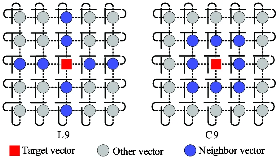
Fig.1 Typical neighborhood structures of CA

The basic model of the evolution rule is as follows.

where Stand St+1denote the cell status at step t and t+1, Ebis the number of an “alive” neighbor needing continuance in its status for an “alive” cell; Fkis the number of an “alive” neighbor needing resurrection for a “dead” cell.

The cellular survival space density is different for different evolution rules and affects the mutual restraint relationship between vectors. The three rules (Rule1: Eb={2,3}, Fk={3}, Rule2: Eb={1,2,3,4}, Fk={4,5,6,7}, and Rule3: Eb={2,4,6,8}, Fk={1,3,5,7}) are utilized for the simulation of stable, periodic and complex states which shall be caught in biological reproduction of confusion.

2.2 Orthogonal crossover operator

The aim of the cross operation is to pass the chunks with excellent properties in the vector to the vector of the next generation, making them excellent in parental vectors. However, the classical DE employs binomial or exponential crossover operator, which obviously can’t obtain above objective in most cases. It is advisable to sample a small but representative sample of all combinations for test[13].

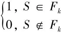
For the above purpose, Lq(nm) is employed as the orthogonal array for m factors and n levels, which has q rows in which every row represents a combination of levels[14]. In this paper, n=2 represents that all factors have two levels: 0 and 1. Based on the level of every factor, the value of a trial vector will be selected from the target vector or its mutant vector in every dimension. m=D is the dimension of the evolutional vector and q is the total number for completion of full test of D factors. The operation is described as the orthogonal crossover, which is shown in Fig.2.

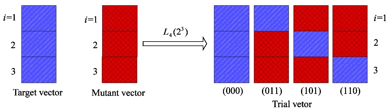
Fig.2 Orthogonal crossover of a 3D vector

In Fig.3 four selected combinations have been shown as black dots illustrating the orthogonality of a three-factor orthogonal array.

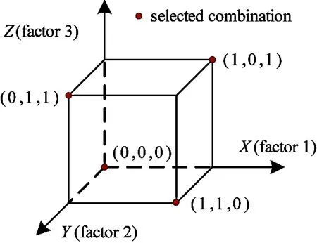
Fig.3 Three-factor orthogonal array

2.3 Description of cDE algorithm

In the cDE algorithm, one cell value of the cellular automata represents the status of the evolutional vector with the same subscript: alive or dead, and only the “alive” vector can be evoluted. The size of the cellular automata is equal to the evolutional population. The proposed cDE algorithm is described as follows:

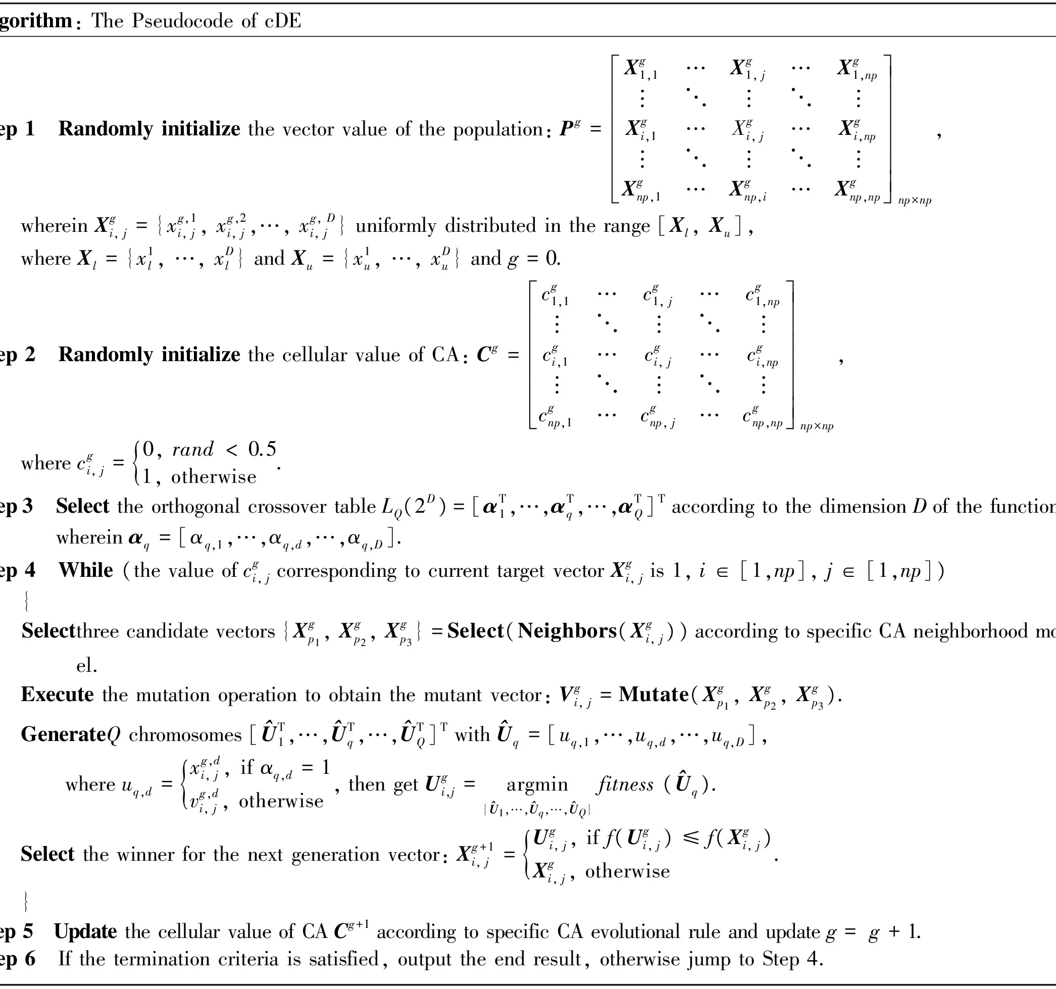
Algorithm：ThePseudocodeofcDEStep1 Randomlyinitializethevectorvalueofthepopulation：Pg=Xg1，1…Xg1，j…Xg1，np︙⋱︙⋱︙Xgi，1…Xgi，j…Xgi，np︙⋱︙⋱︙Xgnp，1…Xgnp，i…Xgnp，npéëêêêêêêùûúúúúúúnp×np， whereinXgi，j={xg，1i，j，xg，2i，j，…，xg，Di，j}uniformlydistributedintherange[Xl，Xu]， whereXl={x1l，…，xDl}andXu={x1u，…，xDu}andg=0．Step2 RandomlyinitializethecellularvalueofCA：Cg=cg1，1…cg1，j…cg1，np︙⋱︙⋱︙cgi，1…cgi，j…cgi，np︙⋱︙⋱︙cgnp，1…cgnp，j…cgnp，npéëêêêêêêùûúúúúúúnp×np， wherecgi，j=0，rand<0．51，otherwise{．Step3 SelecttheorthogonalcrossovertableLQ(2D)=[αT1，…，αTq，…，αTQ]TaccordingtothedimensionDofthefunctions，whereinαq=[αq，1，…，αq，d，…，αq，D]．Step4 While(thevalueofcgi，jcorrespondingtocurrenttargetvectorXgi，jis1，i∈[1，np]，j∈[1，np]) { Selectthreecandidatevectors{Xgp1，Xgp2，Xgp3}=Select(Neighbors(Xgi，j))accordingtospecificCAneighborhoodmod⁃el． Executethemutationoperationtoobtainthemutantvector：Vgi，j=Mutate(Xgp1，Xgp2，Xgp3)． GenerateQchromosomes[＾UT1，…，＾UTq，…，＾UTQ]Twith＾Uq=[uq，1，…，uq，d，…，uq，D]， whereuq，d=xg，di，j，ifαq，d=1vg，di，j，otherwise{，thengetUgi，j=argmin{＾U1，…，＾Uq，…，＾UQ}fitness(＾Uq)． Selectthewinnerforthenextgenerationvector：Xg+1i，j=Ugi，j，iff(Ugi，j)≤f(Xgi，j)Xgi，j，otherwise{． }Step5 UpdatethecellularvalueofCACg+1accordingtospecificCAevolutionalruleandupdateg=g+1．Step6 Iftheterminationcriteriaissatisfied，outputtheendresult，otherwisejumptoStep4．

3 Experimental results and discussions

3.1 Description of benchmark functions

Experiments used to evaluate and compare several DE variants are conducted on a suite of 7 benchmark functions with different characteristics[2]. Functions f1, f2, f4and f5are shift for solving the problem that global optimum lies at the center of the search range. Functions f3and f6are rotated to avoid local optimum lying along the coordinate axes or suffer from global optimum lying at the center of the search range. Function f7is constructed by utilizing some basic problems to obtain one more challenging problem. For all functions, both 10-dimensional (10D) and 30-dimensional (30D) problems are tested. Table 1 outlines the function name, search range and global optimum of 7 benchmark functions.

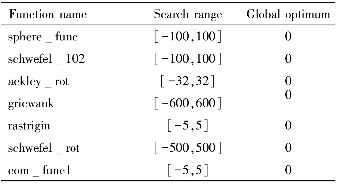
Table 1 Descriptions of 7 benchmark functions

3.2 Parameter setting for comparison

Experiments in this paper are conducted 25 times independently on 7 benchmark functions to compare the proposed cDE with the classical DE, SDE, jDE, DE_Zaharie and SaDE. The control parameters F, CR and NP of above six DE variants are set as used in Ref.[2].

For the proposed cDE algorithm, the orthogonal crossover employs the tailor-made array of the first 10-columns of the orthogonal list L12(211) when the dimension of test problem is 10. In the orthogonal list L12(211), 0 or 1 represents one dimension parameter of a trial vector which is selected from the target vector or its mutant vector of DE. The total number of experiments is 12. The orthogonal crossover is composed of three orthogonal lists at D=10 side by side when the dimension of test problem is 30. The maximum number of function evaluations (FEs) is set to be 100 000 for all benchmark functions. For 12 combinations of levels are used in orthogonal crossover, the FEs of the cDE algorithm is set to be 100 000/12 for the sake of fairness. The cellular evolution rule in cDE in this paper uses Rule2[15]. The neighbor structure of vectors in cDE uses the optimum C9 neighbor model[9].

3.3 Comparison of the final solutions accuracy

In order to demonstrate the effects of CA on improving the performance of DE, cDE is compared with the classical DE algorithm and four kinds of DE variants, then the mean values and standard deviations (Std) of the best values are calculated by the results of 25 independent runs over 7 benchmark functions. Table 2 and Table 3 show the result of benchmark functions at D=10 and D=30 respectively, where the best value for each benchmark function has been shown in boldface.

From Table 2 and Table 3, it can be seen that the performance of cDE is superior to classical DE and four kinds of DE variants. The cDE algorithm obtains smaller mean values even theoretical optimum of all 7 benchmark functions at D=10 and D=30. Therefore it can be concluded that the mechanism of CA on improving the DE is significant.

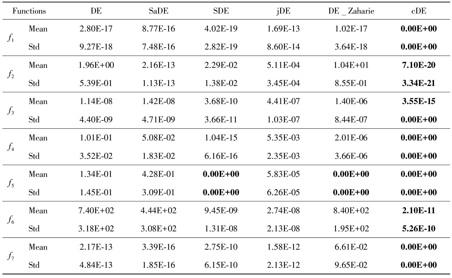
Table 2 The means and standard deviations of 10D funcitons

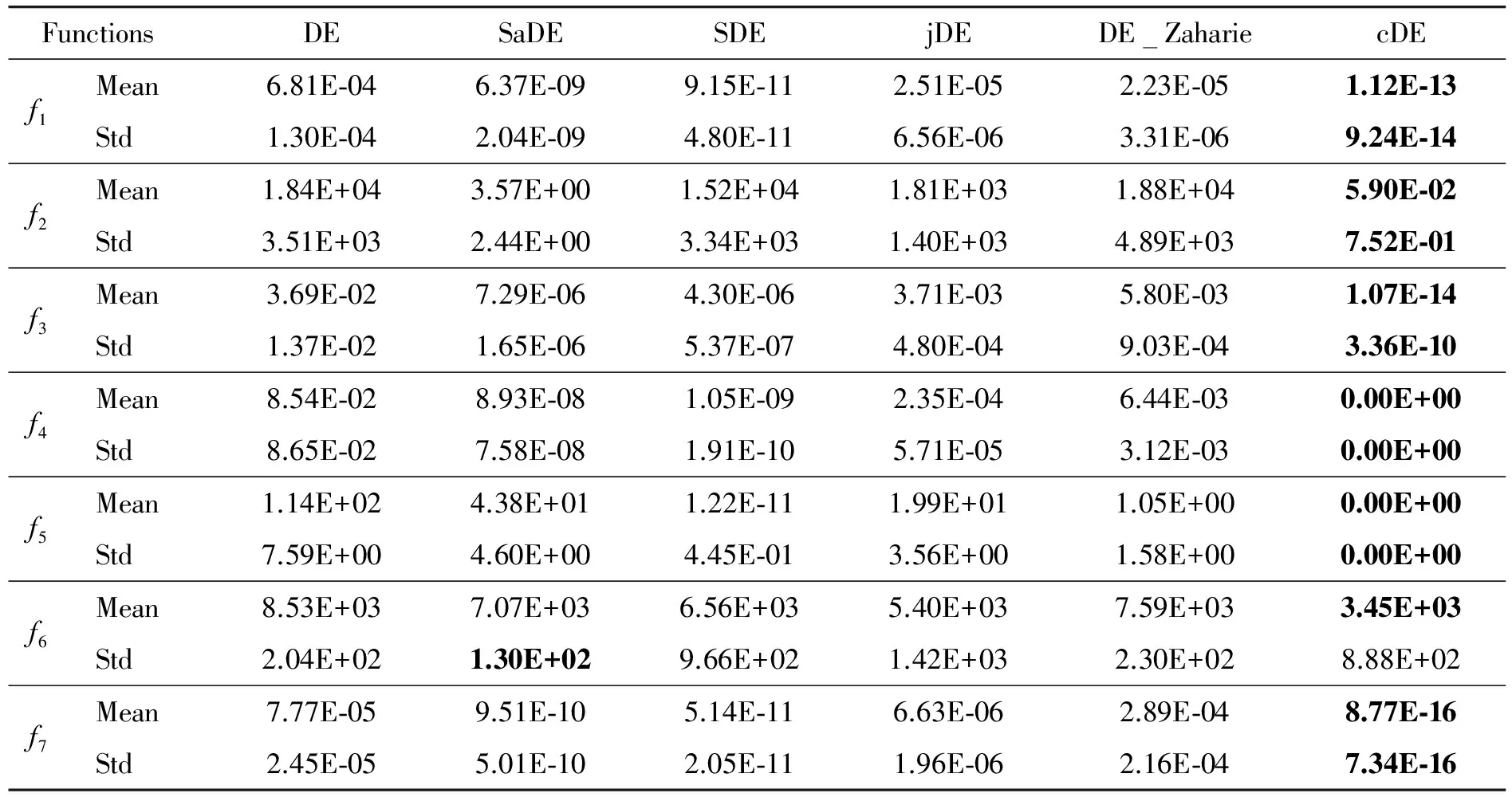
Table 3 The means and standard deviations of 30D functions

Fig.4 and Fig. 5 illustrate the convergence performance in terms of the median run of the best fitness value of the cDE, the classical DE, and four DE variants on 10D and 30D problems, respectively.It can be seen from Fig.4 and Fig.5 that cDE gets little different adaptation values from the classical DE and four DE variants at the initial stage. Furthermore, the convergence performances between cDE and some other DEvariants in Fig.4 show that the cDE always converges faster than others and has access to the optimum more easily than others on most of all 10D functions. Multiple benchmark functions for cDE algorithm have been converged end before 100,000 FEs. What’s more, for the 30D functions, it is greatly difficult to find the global optimum for all DE variants. The cDE algorithm performs better on most problems in Fig.5.

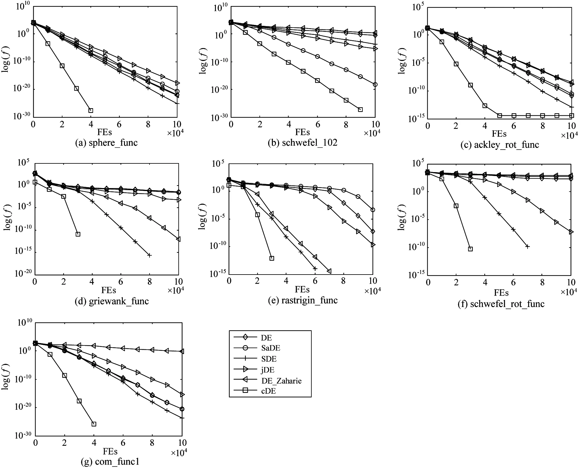
Fig.4 The convergence performances of cDE in comparison with DE variants on 10D functions

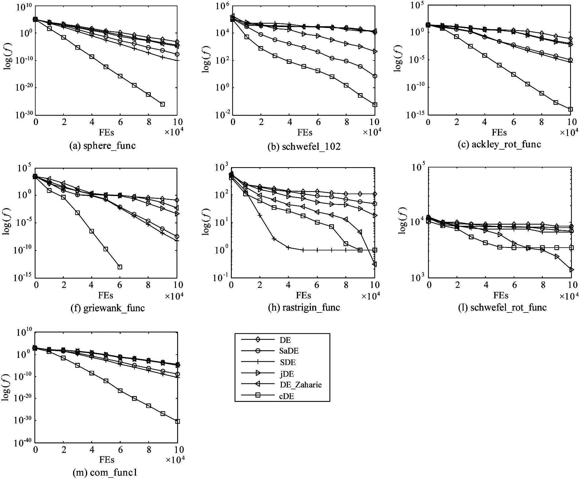
Fig.5 The convergence performances of cDE in comparison with DE variants on 30D functions

3.4 Wilcoxon matched-pairs signed-ranks test

In order to further illustrate the above conclusions, the Wilcoxon matched-pairs signed-ranks test is employed to compare cDE with the classical DE and four kinds of DE variants respectively. Table 4 is the Wilcoxon p-values of the mean data in Table 2 and Table 3.

As can be seen from Table 4, cDE outperforms the classical DE and four kinds of DE variants with the significance level α=0.05 considering independent matched-pairs comparisons at D=10 and D=30.

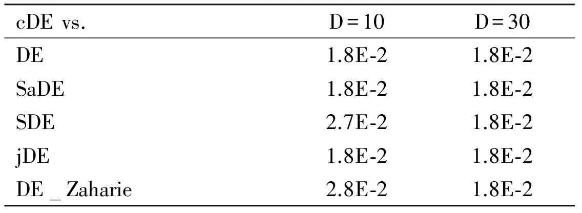
Table 4 p-values of Wilcoxon matched-pairs signed-ranks test

3.5 Convergence analysis

To illustrate the effect of orthogonal crossover operator, the BicDE algorithm has been designed. The only difference between the BicDE algorithm and cDE algorithm is that BicDE algorithm uses the binomial crossover while cDE algorithm uses the orthogonal crossover.

Fig.6 illustrates the convergence characteristics comparison in term of the best fitness value between cDE and BicDE on functions f1～f7at D=10 and D=30. From Fig.6, it can be seen that the convergence rate of cDE is faster than BicDE for all 7 benchmark functions. Accordingly, the cDE algorithm requires smaller FEs than the BicDE algorithm and therefore it has smaller time complexity.

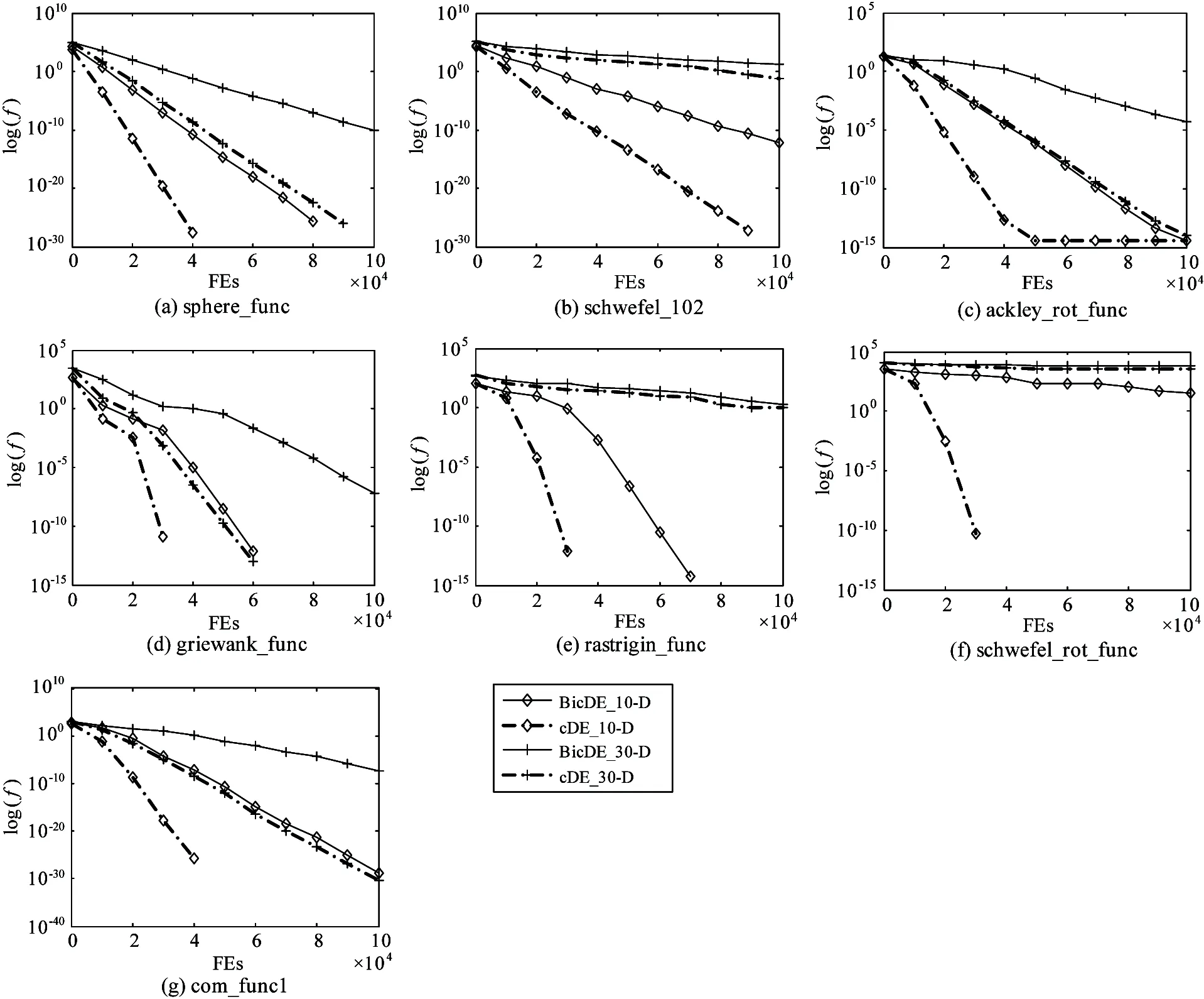
Fig.6 The convergence characteristics of cDE vs BicDE for 7 benchmark functions

The above results confirm two conclusions. The first one is that cDE algorithm can tune the selection pressure by using local search within cellular neighbor structure instead of using its controlling parameters in the classical DE and plenty of cellular evolution rules ensure maintaining the diversity of evolutional population which can avoid falling into local optimum, so the probability of searching the global optimum will increase. The second one is that the orthogonal crossover operator provides repeated trials of multi-element for the cDE algorithm more easily to find the global optimum than those DE variants with binomial crossover and thus helps to accelerate the convergence speed.

4 Conclusions

A novel cDE algorithm without crossover rate is presented, in which those evolutional interactions among vectors are restricted within cellular neighbors while the cell is dynamic evolutionary. The parallel evolution mechanism and cellular neighbor stucture are applied to balance exploration and exploitation tradeoff of DE. The binomial crossover operator is replaced by the orthogonal crossover, which may maintain the population diversity and enhance convergence speed. Through comparing the convergence performance of cDE with the classical DE and four DE variants over a suit of 7 benchmark functions, the simulation results show that the cDE algorithm has better capability of maintaining the population diversity, which can avoid being trapped into the local optimum effectively and has faster convergence speed.

[ 1] Storn R, Price K. Differential evolution-a simple and efficient heuristic for global optimization over continuous spaces. Journal of Global Optimization, 1997, 11(4): 341-359

[ 2] Das S, Suganthan P. Differential evolution: a survey of the state of the art. IEEE Transactions on Evolutionary Computation, 2011, 15(1): 4-31

[ 3] Jia L Y, He J X, Zhang C, et al. Differential evolution with controlled search direction. Journal of Center South University, 2012, 19(1): 3516-3523

[ 4] Alba E, Tomassini M. Parallelism and evolutionary algorithms. IEEE Transactions on Evolutionary Computation, 2002, 6(5): 443-462

[ 5] Michael O, Jimmy M. Predicting and monitoring the evolution of a coastal barrier dune system postbreaching. Jouranl of Coastal Research, 2013, 29(6a): 38-50

[ 6] Alba E, Dorronsoro B. The exploration/ exploitation tradeoff in dynamic cellular genetic algorithms. IEEE Transactions on Evolutionary Computation, 2005, 9(2): 126-142

[ 7] Kim W C K, Man W M, Wan C S. Adding learning to cellular genetic algorithms for training recurrent neural networks. IEEE Transactions on Neural Networks, 1999, 10(2): 239-252

[ 8] Zhang Y, Hu F, Liu Z, et al. Optimization design of truss structure based on synchronous cellular genetic algorithm. In: Proceedings of the 4th International Conference on Intelligent Control and Information Processing, Beijing, China, 2013. 94-97

[ 9] Noman N, Iba H. Cellular Differential Evolution Algorithm. Berlin Heidelberg: Springer, 2011. 293-302

[10] Dorronsoro B, Bouvry P. Differential Evolution Algorithms with Cellular Populations. Berlin Heidelberg: Springer, 2010. 320-330

[11] Noroozi V, Hashemi A, Meybodi M. CellularDE: A Cellular Based Differential Evolution for Dynamic Optimization Problems. Berlin Heidelberg: Springer, 2011. 340-349

[12] Von N, Burks A. Theory of Self-reproducing Automata. Urbana: University of Illinois Press, 1996. 1-6

[13] Zamani R. Integrating iterative crossover capability in orthogonal neighborhoods for scheduling resource-constrained projects. Evolutionary Computation, 2013, 21(2): 341-360

[14] Li H, Zhang L, Jiao Y C. Solution for integer linear bilevel programming problems using orthogonal genetic algorithm. Journal of Systems Engineering and Electronics, 2014, 25(3): 443-451

[15] Lu Y M, Li M, Li L. The cellular genetic algorithm with evolutionary rule. Acta Electronica Sinica, 2010, 38(7): 1603-1607

10.3772/j.issn.1006-6748.2017.04.012

①Supported by the National Natural Science Foundation of China (No. 61501186), the Jiangxi Province Science Foundation (No. 20171BAB202001) and the Visiting Scholar Foundation of Jiangxi Province Young and Middle-aged University Teachers’ Development Program ([2016], No. 169).

②To whom correspondence should be addressed. E-mail: brandy724@sina.com

on Jan. 6， 2017

his Ph.D degree from the School of Communication and Information Engineering of Shanghai University in 2015 and his M.S. degree from the School of Electrical and Electronic Engineering of East China Jiaotong University in 2007. His research addresses the optimization technology in the receiver design of wireless communication, such as convex optimization and multi-objective optimization.