Guo Chen (郭 晨), Liang Jiarong, Leng Ming, Peng Shuo

(*School of Electronic and Information Engineering, Jinggangshan University, Ji’an 343009, P.R.China) (**School of Computer and Electronic Information, Guangxi University, Nanning 530004, P.R.China) (***Department of Computer Science and Technology, Tsinghua University, Beijing 100084, P.R.China)

A novel conditional diagnosability algorithm under the PMC model①

Guo Chen (郭 晨)*, Liang Jiarong②, Leng Ming***, Peng Shuo*

(*School of Electronic and Information Engineering, Jinggangshan University, Ji’an 343009, P.R.China) (**School of Computer and Electronic Information, Guangxi University, Nanning 530004, P.R.China) (***Department of Computer Science and Technology, Tsinghua University, Beijing 100084, P.R.China)

Conditionally t-diagnosable and t-diagnosable are important in system level diagnosis. Therefore, it is valuable to identify whether the system is conditionally t-diagnosable or t-diagnosable and derive the corresponding conditional diagnosability and diagnosability. In the paper, distinguishable measures of pairs of distinct faulty sets with a new perspective on establishing functions are focused. Applying distinguishable function and decision function, it is determined whether a system is conditionally t-diagnosable (or t-diagnosable) or not under the PMC (Preparata, Metze, and Chien) model directly. Based on the decision function, a novel conditional diagnosability algorithm under the PMC model is introduced which can calculate conditional diagnosability rapidly.

the PMC (Preparata, Metze, and Chien) model, conditionally t-diagnosable, conditional diagnosability, conditional diagnosability algorithm

0 Introduction

With the continuous development of large-scale integration, multiprocessor computer systems can consist of hundreds of processors. However, the high complexity of those systems may threaten their reliability. To resolve this issue, in 1967, Preparata, Metze, and Chien presented the definition of system level diagnosis and proposed a so-called PMC model and t-diagnosable[1]. In 1992, Sengupta and Dahbura proposed that the most important necessary and sufficient condition for t-diagnosable was that each pair of distinct faulty sets should be distinguishable, provided the number of faulty vertices was no more than t[2].

Lai, et al.[3]introduced the conditional diagnosability based on the assumption that all neighbors of any processor in a multiprocessor system could not be fault simultaneously. A system is conditionally t-diagnosable if each pair of conditional faulty sets is distinguishable. Thus far, distinguishability of a pair of distinct faulty sets is widely adopted in the study of t-diagnosable[2,4,5], conditionally t-diagnosable[3,5-9], strong diagnosability[5,9]and g-good-neighbor conditional t-diagnosable[10]. However, lacking of distinguishable measures has caused bad influence.

In this paper, distinguishable measures of pairs of distinct faulty sets with a new perspective on establishing functions is focused. After a distinguishable function and a decision function are constructed, how to identify whether a system is conditionally t-diagnosable (t-diagnosable) or not under the PMC model is studied. Finally, a novel algorithm is given to derive conditional diagnosability under the PMC model.

1 Preliminaries

A multiprocessor computer system consisting of n processors is modeled as a graph where each vertex represents a processor and each edge represents a link. Let G(V, E) be such a graph. An edge (u, v)∈E(G), with u, v∈V(G), is a test edge of G(V, E), which represents a test performed by u on v. The outcome of edge (u, v), denoted by σ(u, v), is “0” if u evaluates v as a pass and “1” if u evaluates v as a fault. An outcome is reliable only if the tester is fault-free. The collection of all test outcomes in G(V, E) is called a syndrome, denoted by σ. Each vertex has two states: fault-free and faulty. If vertex u is identified as fault-free, then denoted by u=0; otherwise u=1.

In the PMC model, each vertex u is able to test another vertex if there is a link between them. The outcome of a test performed by a fault-free tester is 1 (respectively, 0) if the tested vertex is faulty (respectively, fault-free), whereas the outcome of a test performed by a faulty tester is unreliable. Table 1 summarizes the invalidation rules for the PMC model.

Table 1 Invalidation rules for the PMC model

Some known results about faulty set and t-diagnosable are listed below.

Definition 1[4]: A subset F⊆V(G) is called a faulty set of a given syndrome σ, for any (u,v)∈E(G) and u∈V(G)-F, σ(u,v)=0 if v∈V(G)-F, σ(u,v)=1 if v∈F.

For a given syndrome σ, a faulty set F⊆V(G) is said to be consistent with σ if F can produce σ. Let σ(F) represent the set of syndromes which can be produced if F is the set of faulty vertices.

Definition 2[1]: A system is a t-diagnosable one if and only if, for a given syndrome σ, all the faulty vertices can be identified that the number of faulty vertices are not more than t.

Definition 3[2]: Two distinct faulty sets F1and F2are said to be indistinguishable if σ(F1)∩σ(F2)≠Ø; otherwise, (F1, F2) is distinguishable.

According to Definition 2 and 3, the following two lemmas about t-diagnosable are proposed.

Lemma 1[4]: For a pair of distinct faulty sets F1and F2, with F1⊆V(G) and F2⊆V(G), (F1, F2) is distinguishable if there exists at least one test from V(G)-(F1∪F2) to F1ΔF2. Operator Δ implies exclusive-or (XOR). Hence, F1ΔF2=(F1-F2)∪(F2-F1). The operator || implies cardinality. Then, |F1| is the cardinality of F1.

Lemma 2[2]: A system is t-diagnosable if each pair of distinct faulty sets F1and F2is distinguishable, provided that |F1|≤t and |F2|≤t.

Diagnosability is an important measure of self-diagnostic capability. The diagnosability of system G is the maximum value of t such that G is t-diagnosable, written as t(G).

Motivated by the deficiency of classical measurement of diagnosability, Lai, et al. presented conditional diagnosability by claiming the property that each vertex had at least one fault-free neighbor[3]. Then, they introduced some useful definitions and lemmas as follows.

Definition 4[3]: Faulty set F⊆V(G) is a conditional faulty set only if every vertex of the system has at least one fault-free neighbor.

Lemma 3[3]: A system is conditionally t-diagnosable if each pair of distinct conditional faulty sets (F1, F2) is distinguishable, with |F1|≤t and |F2|≤t.

Definition 5[3]: The conditional diagnosability of system G is the maximum value of t that G is conditionally t-diagnosable, denoted as tc(G).

In this paper, an undirected diagnosable system is adopted, which assumes that every test edge is bidirectional. The undirected diagnosable system is a special diagnosable system. An arbitrary edge (u,v) of an undirected diagnosable system implies that u can test v and v can test u too.

2 Distinguishable measure of pairs of distinct faulty sets

As mentioned above, t-diagnosable and conditionally t-diagnosable are closely related to the distinguishability of pairs of distinct faulty sets. Therefore, an interesting question arises here: how to identify whether two distinct faulty sets are distinguishable or not. In this section, some important theorems and lemmas about distinguishable measures of two distinct faulty sets will be presented.

Theorem 1: Let F1and F2be two distinct faulty sets of an undirected diagnosable system, (F1, F2) is distinguishable, then there exists at least one undirected edge (u, v), such (u+v)|F1+(u+v)|F2=1. (u+v)|Fxis the sum of u and v when Fxis the set of faulty vertices, (u+v)|Fx=(u)|Fx+(v)|Fx, (u)|Fx=0 if u∉Fx, and (u)|Fx=1 if u∈Fx. According to the definition of (u+v)|Fx, (u+v)|F1=1 (or (u+v)|F2=1) implies that u+v=1, which means one of {u,v} is fault-free and the other is faulty, when F1(or F2) is the current faulty vertices set.

Proof: This theorem is proved by contradiction. For each undirected edge (u,v) of the system, it is assumed (u+v)|F1+(u+v)|F2≠1. Without loss of generality, there exists 7 cases. As shown in Table 2, only case 2 lacks the possibility of satisfying σ(u,v)|F1=σ(u,v)|F2and σ(v,u)|F1=σ(v,u)|F2, which means σ(F1)∩σ(F2)=Ø.

According to (u+v)|F1+(u+v)|F2≠1, case 2 will not appear in the system. Therefore, the system has the possibility of satisfying σ(u,v)|F1=σ(u, v)|F2and σ(v,u)|F1=σ(v,u)|F2, which implies σ(F1)∩σ(F2)≠Ø. According to Definition 3, (F1, F2) is an indistinguishable pair of faulty sets, which contradicts the assumption. The theorem follows.

It is easy to prove that (u+v)|F1+(u+v)|F2=1 is another form of the existence of at least one test edge from V-(F1∪F2) to (F1△F2). Therefore, Theorem 1 is also proved by Lemma 1.

Table 2 The value of (u+v)|F1+(u+v)|F2underall possible scenarios

Case 1

Case 2

Case 3

Case 4

Case 5

Case 6

Case 7

According to Theorem 1, an important distinguishable function is presented which can identify whether a pair of faulty sets is distinguishable or not.

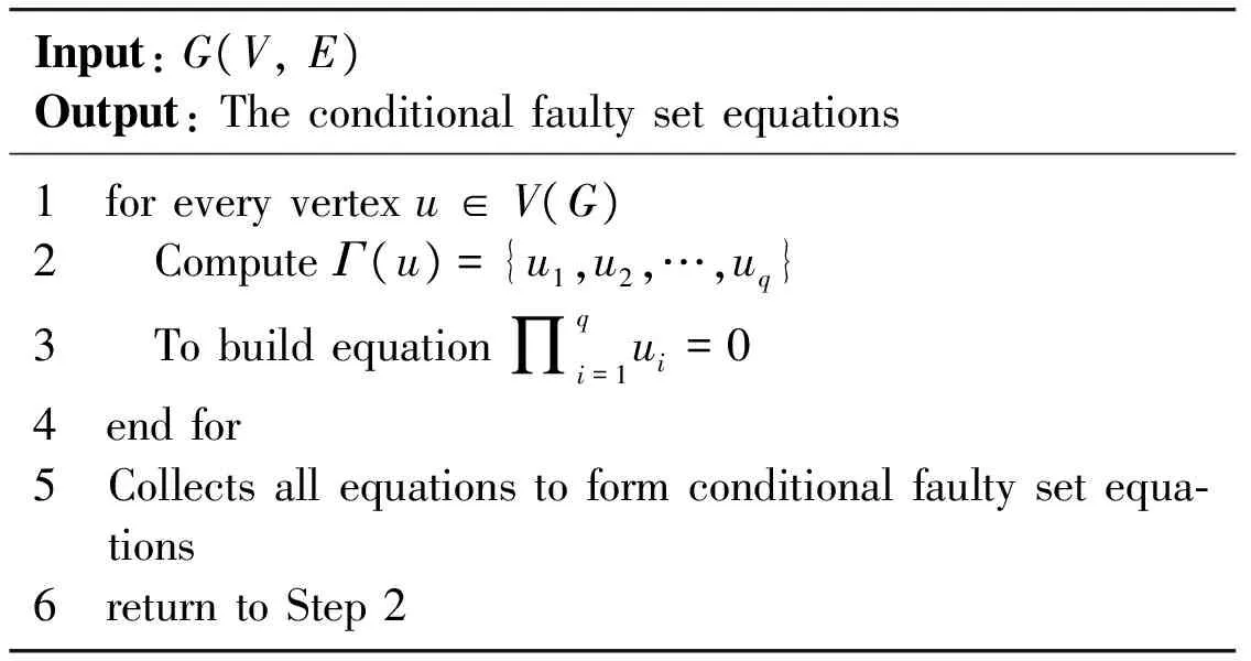
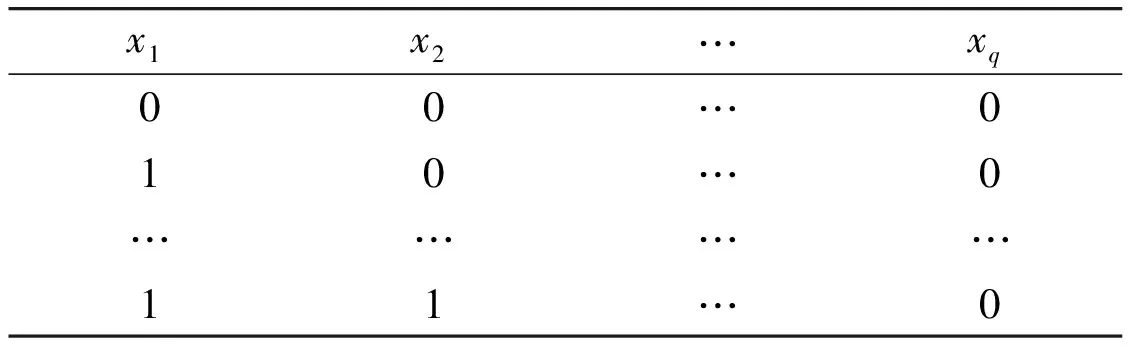
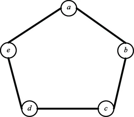
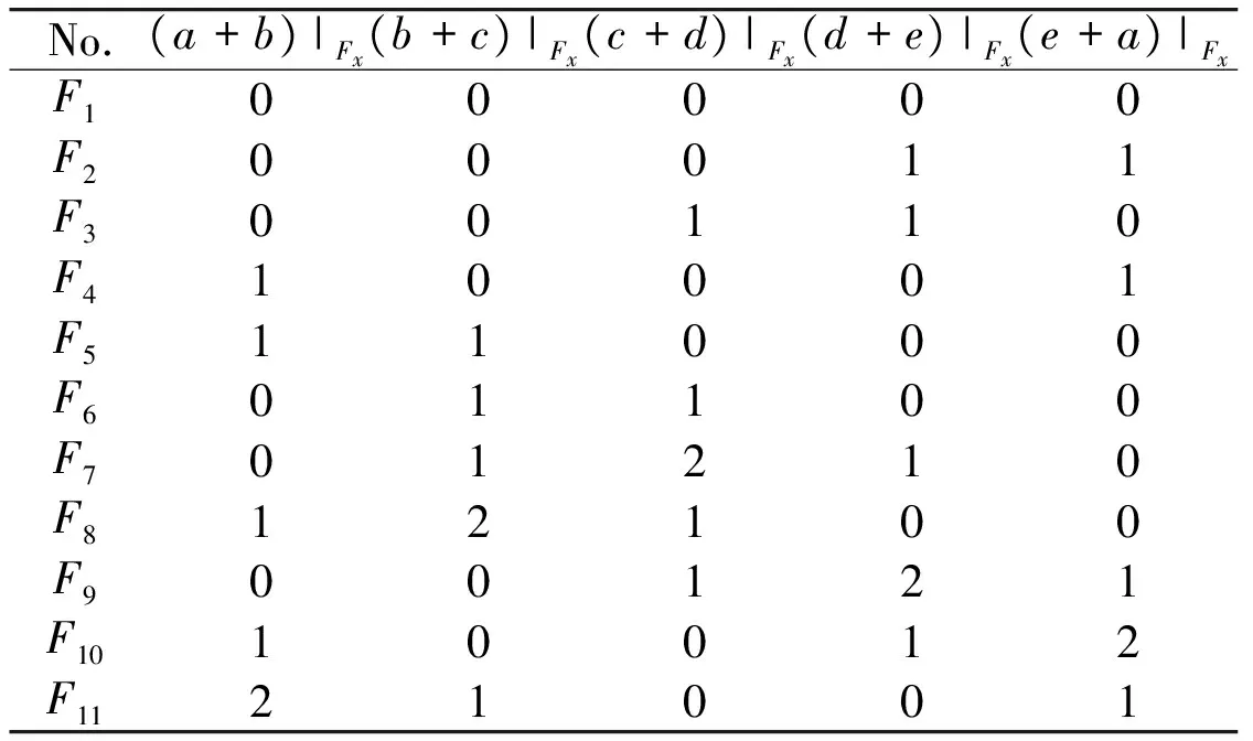
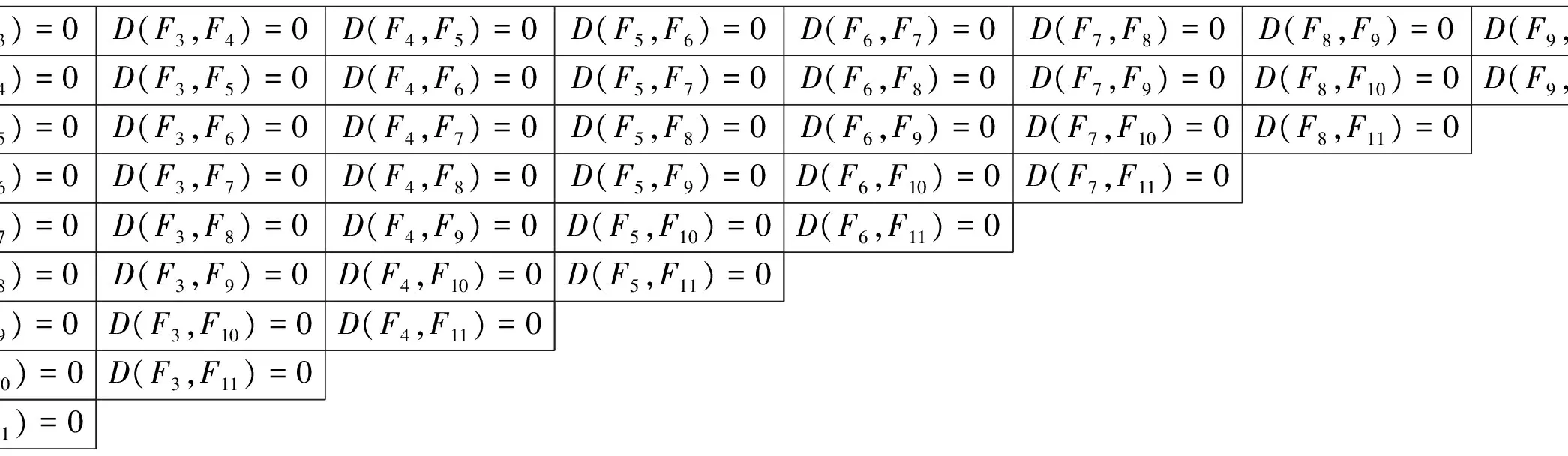
According to Definition 6, D(Fi, Fj)=D(Fj, Fi) is got. To avoid double-counting, i

Lemma 4: D(F1,F2)=0 represents that (F1, F2) is distinguishable; otherwise, (F1, F2) is indistinguishable.

According to Lemma 2 and Lemma 3, t-diagnosable and conditionally t-diagnosable are tied to distinguishability of pairs of distinct faulty sets and conditional faulty sets, respectively.

Next, a decision function will be provided which can decide whether the system is t-diagnosable (or conditionally t-diagnosable).

Lemma 5: J(F1,F2,…,Fm)=0 represents the fact that the system is t-diagnosable (or conditionally t-diagnosable), where F1,F2,…,Fmare all the possible faulty sets (or conditional faulty sets) with |F1|,|F2|,…,|Fm|≤t; otherwise, the system is not t-diagnosable (or conditionally t-diagnosable).

Proof: By Definition 7, J(F1,F2,…,Fm)=0 means D(Fi, Fj)=0 for 1≤i

The decision function J(F1,F2,…,Fm) can be used in both t-diagnosable systems and conditionally t-diagnosable systems. The only difference is whether F1,F2,…,Fmare all the possible faulty sets or all the possible conditional faulty sets.

3 A novel conditional diagnosability algorithm under the PMC model

The conditional diagnosability algorithm under the proposed PMC model is based on Theorem 1 and decision function J(F1,F2,…,Fm). The effectiveness of this conditional diagnosability algorithm has been confirmed by Lemma 5. Above all, all the possible conditional faulty sets of the system must be derived. Then, the decision function J(F1,F2,…,Fm) is called to identify whether the system is conditionally t-diagnosable or not and then obtain conditional diagnosability. The new algorithm can be outlined as follows:

Step 1: Construct conditional faulty set equations.

For each vertex u∈V, we set Γ(u)={u′∈V|(u,u′)∈E}. According to the definition of conditional diagnosability, Γ(u) has at least one fault-free neighbor that can be denoted by Γ(u)=u1u2…uq=0. The equations of all the vertices in the system compose the conditional faulty set equations.

Step 1 can be described by the following pseudocode.

Input：G(V，E)Output：Theconditionalfaultysetequations1 foreveryvertexu∈V(G)2 ComputeΓ(u)={u1，u2，…，uq}3 Tobuildequation∏qi=1ui=04 endfor5 Collectsallequationstoformconditionalfaultysetequa⁃tions6 returntoStep2

Step 2: Convert each equation of the conditional faulty set equations into a relational table.

For example, the equation x1x2…xq=0 means that there exists at least one vertex “0”. The relational table corresponding to x1x2…xq=0 is Table 3, which consists of 2q-1 tuples.

Table 3 The relational table corresponds to x1x2…xq=0

Step 2 can be described as follows:

Input：ConditionalfaultmodelequationsOutput：RelationaltablesX1，X2，…，Xm1 foreveryequationofequations2 TransformequationintoarelationtableXi3 i=i+14 endfor5 returntoStep3

Step 3: Derive all the possible conditional faulty sets.

After all the conditional faulty set equations have been converted into relational tables, all the possible conditional faulty sets in this step will be derived. Let all of the relational tables be X1, X2,…, Xr.

First of all, empty relational table X is defined. If relational tables X and X1have one or more fields in common, then the two tables are joined as a new relational table X by natural join (▷◁), denoted by X=X▷◁X1, otherwise, they are joined by Cartesian product (×), denoted by X=X×X1. Repeat this step from X2to Xr. The final new relational table X is the set of all the possible conditional faulty sets, denoted by X={F1, F2,…,Fm}.

The pseudocode of this step is described as follows:

Input：RelationaltablesX1，X2，…，XrOutput：AllthepossibleconditionalfaultysetsX1 forifrom1tor2 IFthereexistscommonfieldsbetweenXandXi3ThenX=X▷◁Xi4ElseX=X×Xi5 endif6 endfor7 returntoStep4

Step 4: Calculate the sum of the two adjacent vertices of each undirected test edge under different conditional faulty sets and D(Fi,Fj).

The pseudocode of this step is given below.

Input：AllthepossibleconditionalfaultysetsXOutput：Thesumofthetwoadjacentverticesofeachundi⁃rectedtestedgeunderdifferentconditionalfaultysetsandD(Fi，Fj)，1≤i

Step 5: Call the decision function J(F1, F2,…,Fp) to determine whether the system is conditionally t-diagnosable or not and derive tc(G).

Let all those conditional faulty sets which have less than i faulty vertices be F1, F2,…, Fp. J(F1, F2,…, Fp)=0 represents the system is conditionally t-diagnosable, with t=i. tc(G) is the maximum value of t.

Step 5 can be described by the following pseudocode.

Input：D(Fi，Fj)，1≤i

Illustrated by the example of Fig.1, conditional faulty set equations can be constructed as Eq.(1) then to obtain all the relational tables as shown in Table 4. Finally, the new relational table X can be got by X=X1×X2▷◁X3▷◁X4▷◁X5. The result of X is shown in Table 5.

As shown, there are 11 conditional faulty sets, where F1has no faulty vertex, each conditional faulty set of {F2, F3,…, F6} has only one faulty vertex, and each conditional faulty set of {F7, F8,…, F11} has two faulty vertices. The maximum number of faulty vertices of all the possible conditional faulty sets is 2. That is to say, tc(G)≤2. The sums of the two adjacent vertices of each undirected test edge under different conditional faulty sets are shown in Table 6. And D(Fi, Fj)=0 for 1≤i

Fig.1 A system consisting of 5 vertices

(1)

Table 4 Relational tables corresponding to Eq. (1)

4 Conclusion

Conditional diagnosability is a new measure of diagnosability which claims that each vertex has at least one fault free neighbor. Therefore, all the fault processors can be identified if the number of fault processors in a system is less than the conditional diagnosability and any faulty set cannot contain all neighbors of any processor . As a result a conditional diagnosability algorithm is more important, which can determine conditional diagnosability of any system. With the continuous development of large-scale integration, multiprocessor systems may have hundreds of processors, especially in supercomputer systems,high-performance parallel computing systems and grid systems, which areusually based on an underlying bus structure, or a kind of interconnection networks. However, the high complexity of these systems may threaten their reliability. Hence, an efficient conditional diagnosability algorithm has important theoretical significance and application value, which can be used to evaluate the reliability of multiprocessor systems.

Table 5 All the conditional faulty sets in X

Table 6 The sums of the two incident vertices

Table 7 The results of D(Fi, Fj), for 1≤i

In this paper, the distinguishable measure of pairs of distinct faulty sets have be investigated. By theoretical deduction, an effective decision function J(F1,F2,…,Fm) and a novel conditional diagnosability algorithm are presented successfully which can identify whether the system is conditionally t-diagnosable or not directly and obtain tc(G) conveniently under the PMC model.

[ 1] Preparata F P, Metze G, Chien R T . On the connection assignment problem of diagnosable systems. IEEE Transactions on Electronic Computers, 2006, 16(6): 848-854

[ 2] Sengupta A, Dahbura A T. On self-diagnosable multiprocessor systems: diagnosis by the comparison approach. IEEE Transactions on Computers, 1992,41(11):1386-1396

[ 3] Lai P L, Tan J J, Chang C P, et al. Conditional diagnosability measures for large multiprocessor systems. IEEE Transactions on Computers,2005, 54(2):165-175

[ 4] Dahbura A T, Masson G M. An 0(n2.5) fault identification algorithm for diagnosable systems. IEEE Transactions on Computers, 1984, C-33(6):486-492

[ 5] Zhu Q, Guo G D, Wang D. Relating diagnosability, strong diagnosability and conditional diagnosability of strong networks. IEEE Transactions on Computers, 2014,63(7):1847-1851

[ 6] Yang M C. Analysis of conditional diagnosability for balanced hypercubes. In: Proceedings 2012 International Conference on IEEE, of the Information Science and Technology, Wuhan, China, 2012. 651-654

[ 7] Xu M, Thulasiraman K, Hu X D. Conditional diagnosability of matching composition networks under the PMC model. IEEE Transactions on Circuits and Systems II: Express Briefs, 2009, 56(11): 875-879

[ 8] Zhu Q. On conditional diagnosability and reliability of the BC networks. The Journal of Supercomputing, 2008, 45(2):173-184

[ 9] Hsieh S Y, Tsai C Y, Chen C A. Strong diagnosability and conditional diagnosability of multiprocessor systems and folded hypercubes. IEEE Transactions on Computers, 2013, 62(7):1472-1477

[10] Peng S L, Lin C K, Jimmy J M, et al. The g-good-neighbor conditional diagnosability of hypercube under PMC model. Applied Mathematics and Computation, 2012,218(21):10406-10412

Guo Chen, was born in 1979. He is a Ph.D candidate of Guangxi University. He received his M.S. degree in computer science from Guanxi University in 2005. He received his B.S. degree of computer science from Beijing Business and Technology University in 2001. His research interests include artificial intelligence and interconnection network.

10.3772/j.issn.1006-6748.2017.04.006

①Supported by the National Natural Science Foundation of China (No. 61562046) and Science and Technology Project of Jiangxi Provincial Education Department (No. GJJ150777, GJJ160742).

②To whom correspondence should be addressed. E-mail: 13977106752@163.com

on Mar. 6， 2017**