1 气候预测理论与方法

1.1 南亚高压强度和位置变化的2个主导模态及其形成机制

揭示了5月南亚高压强度和位置变化的2个主导模态，提出了ENSO的持续性和印度洋的海温作用对上述2种模态的影响和机理。5月南亚高压的形态变异将亚洲夏季风爆发的各个阶段连接成一个完整接续的动力过程。本工作根据观测资料定义了5月南亚高压的强度、东西伸脊点和脊线位置，并利用主成分分析（PCA）方法提取了5月南亚高压的主导模态。结果表明，5月南亚高压的年际变化具有两种主导模态：一种是强度模态，表现为南亚高压的强度和纬向跨度的一致变化，另一种是经向位置模态，表现为南亚高压脊线经向位置的年际差异。

虽然5月南亚高压的强度和经向位置模态都受前冬ENSO事件影响，但ENSO事件影响南亚高压各主导模态的物理过程却并不相同。尽管前冬ENSO事件在春季衰减，其信号仍能通过“大气桥”转移到热带印度洋地区，并通过印度洋海温异常（SSTA）来影响周边的大气环流异常。观测和数值模拟结果表明，印度洋和太平洋SSTA影响南亚高压主导模态的相对贡献却与ENSO事件在春季的衰减快慢有关。当前冬ENSO事件在春季衰减较快时，其引起的5月印度洋SSTA能够改变亚洲南部局地对流强度，其激发的Rossby波响应位于印度西南部上空，令南亚高压强度模态发生变化；当前冬ENSO事件衰减较慢时，5月印度洋SSTA始终受ENSO引起的大气环流异常影响，因此来自热带太平洋的SSTA通过改变亚洲南部地区的垂直运动，进而调整局地经向温度梯度，并影响南亚高压的经向位置模态。本研究结果说明，除ENSO事件的冷、暖位相外，它对亚洲夏季风高空环流的影响还随其在春季的演变过程不同而改变（图1）。（刘伯奇，祝从文）

1.2 2015/2016年超强El Niño事件次年盛夏西太平洋副高异常偏弱的成因

以往研究认为，当前冬发生了El Niño事件后，次年夏季西太平洋副高将异常偏强，这主要和El Niño引起的西北太平洋海—气相互作用和热带印度洋海盆尺度异常增暖有关。但最新的观测指出，在2015/2016年冬季超强El Niño事件发生后，2016年7、8月西太平洋副高异常偏弱，这与已有的ENSO-西太平洋副高关系不符。本研究通过资料分析和数值试验表明，与历史事件相比，2015/2016年冬季超强El Niño事件衰减更快，令次年夏季印度洋无法充分加热，因此印度洋暖SSTA无法在盛夏维持，从而削弱了印度洋暖SSTA通过局地纬向环流异常来加强西太平洋副高的作用。同时，来自中纬度的对流层中上部波列在2016年夏季能够南传到达西太平洋地区，进一步削弱了西太平洋副高的强度。（刘伯奇，祝从文，苏京志，华丽娟）

1.3 全球变暖已由趋缓期转为加速期

自1999年至2012年间，全球平均表面温度（GMST）升温速率较先前几十年偏低，此即“全球变暖停滞/趋缓”现象。但“变暖趋缓”何时结束，此前存在较大争议。然而在2014年、2015年和2016年GMST相继创下历史最高记录。我们研究表明，GMST这种“三级跳”式破纪录攀升现象尚属首次，这标志着全球变暖由“趋缓期”转为“加速期”。对排名前十的年平均高温记录在各年代的发生频次（NT10）统计显示，NT10在1960年代后节节攀升，即便是在“趋缓期”也显著增加，这表明全球变暖的持续增温趋势始终没有改变。就机理而言，太平洋年代际振荡（PDO）自2013年开始由负位相转为正位相，这有利于全球表面温度升温速率重新加速。变暖趋缓期间，海洋吸收了更多的热量，这些热量的释放将导致气温升高。2014/2015年超强厄尔尼诺进一步加剧了全球温度升高。厄尔尼诺对滞后3个月GMST的影响最显著，因此冬季年（6月至次年5月）平均的GMST年际变率与NINO3区温度有着很好的关联。然而，导致这几次破纪录高温的最根本的驱动力，仍来源于全球变暖持续升温的背景趋势。对未来几十年情景预估表明，全球气温将会持续维持历史高位，破纪录历史高温将频繁出现，并形成一种新常态（图2）。（苏京志）

1.4 天山中部地区夏季降水量变化的气候特征

研究了天山中部地区夏季降水量日变化的气候特征。基于逐小时降雨量数据和卫星观测所得对流指数的分析表明：此区域有3个显著特征，即南部山区的清晨高峰值，山区傍晚的高峰值，以及北部山区夜间的高峰值。进一步分析了这些日变化特征之间的关系。通过定义区域降水事件（RRE），记录每个RRE的初始位置。在南部盆地南部地区，山脉南部的早期降雨是由局地所引起的。山区傍晚的降水峰值和北部山区的夜间降水峰值都受到了山区降雨事件的影响。这些降水事件在下午出现在山区，其中一些会向北移动，导致北部盆地的夜间降雨。山区下午对流触发以及在南部盆地的清晨降水都与山脉周围的昼夜变化的风和热力学条件有关。在山脉（南部盆地）的对流形成之前的中午（晚上），热力不稳定相伴随的低层辐合对流出现（图3）。（李建）

1.5 青藏高原低涡对西南涡生成的影响

西南涡产生于青藏高原东侧的我国西南地区，定义在700 hPa上，是影响我国西南乃至东部广大地区降水的重要天气系统。青藏高原低涡是产生于青藏高原主体上的500 hPa天气系统，它们的移出能够对西南涡的活动产生影响。然而，目前关于移出的青藏高原低涡对西南涡生成的影响的研究很少。本文基于FNL资料对2000—2011年移出型高原低涡对西南涡的生成的影响进行了研究。研究选择了3类过程：第1类，有高原低涡伴随下的西南涡生成过程；第2类，仅有高原低涡，没有西南涡生成过程；第3类，没有高原涡伴随下的西南涡生成过程。每个过程包含9个个例，研究分别对这3个过程进行了分析，并进一步通过对比指出了移出型高原低涡在西南涡生成过程中的作用。结果指出，凝结潜热加热对西南涡是西南涡生成的决定性因素，而移出型高原低涡能够在西南地区创造更加有利的降水条件，从而有利于西南涡的生成。有高原低涡伴随下的西南涡生成后，强度更大，维持时间更长。但是高原低涡并非西南涡产生的充分条件，强烈的西南气流及相应的水汽输送对西南涡对的产生起到了关键作用。（李论）

1.6 中国夏季极端暖事件的类型分析

根据白天最高温度和夜间最低温度的极端性及二者的组合情况，将中国夏季的暖事件细分为3种互不重叠的子类，即独立白日型、独立夜间型及混合型。这些子类的变化与传统定义中的暖日、暖夜事件的变化在趋势的显著性、强度甚至是符号正负等方面均存在明显差异，这些差异在包含极端白天温度的子类中尤为明显。按照上述分类，一些在传统定义中被忽视的显著变化被成功挖掘出来。如，独立白日型的支配地位正在逐渐减弱，而混合型事件和独立夜间型事件逐渐演化成主要的暖事件类型。这两类暖事件具体表现为频次显著增长、持续时间显著延长、影响范围显著扩张，并且强度越强的事件增强的幅度越大。（陈阳，翟盘茂）

1.7 近20年中国东部地区的持久且较强的变暖减缓现象

在1997年以来，中国东部地区经历了一次变暖减缓过程，主要表现为早冬的最低温度的显著变冷。通过随机组合起始年份，发现中国东部的“优势变暖减缓期”发生在1998—2013间，这段时间内的区域平均最低温度变冷的趋势最强并且达到显著变冷的站点数最多。对变暖减缓最为敏感的区域主要位于华北、江淮地区和华南，这些敏感区的显著变冷趋势一直持续到了2016年。这种持续的变暖减缓使得严重的冷事件在上述地区频发。达到如此强度且持久的变暖减缓期在过去50年间都不曾发生，因此可以被视为气候变暖大背景下的一个“奇异值”（图4）。（陈阳，翟盘茂）

1.8 全球增暖导致盛夏华东高温事件的发生概率增大

包括热浪在内的极端气候事件的频率、强度和持续时间正在发生着变化。极端气候事件极容易引发灾害，对极端气候事件的归因是气候学界关注的热点方向，这其中的一个挑战性问题是对单一极端气候事件的归因，原因在于单一极端事件既可能受到气候变化的影响，又包含自然变率的信号。2013年7—8月，我国华东地区经历了1951年以来持续时间最长（长于40天）、强度最高（区域最高温度44.1℃）的热浪事件。围绕着这次高温事件的归因问题，基于超级集合归因模拟试验和耦合模式集合模拟结果，研究了气候变化和自然内部变率对该极端事件的影响，研究发现大气自然变率和人类活动对这次热浪事件均有贡献；与这次热浪事件直接相关的大气环流型，表现为华东地区上空的异常正高压，这种高压型自身因大气内部变率而产生；人类活动影响显著增加了类似2013年盛夏极端高温事件的发生概率（图5）。（马双梅）

2 气候系统模式研发

2.1 气候系统模式简介

中国气象科学研究院气候系统模式（CAMS-CSM）得到进一步发展完善。现有版本CAMS-CSM包含了先进的大气模式ECHAM5（v5.4）、海洋模式MOM4、海冰模式SIS、陆地表面模式CoLM和FMS耦合器等组成分量。在大气模式ECHAM5中引入了欧拉型“两步保形平流方案”（TSPAS），并采用了跳点差分算法，模拟结果显示新方案对东亚地区降水特别是青藏高原大地形周边降水有明显改善，显著降低了陡峭地形区高海拔区域的降水。同时将大气模式的辐射模块替换为BCC_RAD辐射方案，模拟结果显示新方案显著改善了大气顶的辐射平衡，同时明显改善了对东亚地区短波云辐射状况的模拟。在各模块通量耦合过程中，针对大气模式中半隐式垂直扩散方案发展了一套新的守恒的通量计算和插值算法，保持了海—气和冰—气界面的能量守恒以及模式的稳定积分。通过改进海—陆边界格点的通量算法，保证了海—陆边界格点的通量守恒，模式积分过程中海温和海冰的长期变化趋势明显减弱。利用该版本CAMS-CSM，对工业革命前控制试验和历史试验进行积分模拟。通过分析上述试验结果，发现该版本CAMS-CSM很好地再现了气候平均状态和主要气候系统的季节周期，包括海表温度、降水、海冰范围和海洋温跃层等要素特征，并能合理再现主要的气候变率模态，如Madden-Julian振荡（MJO）、ENSO、东亚夏季风（EASM）以及太平洋年代际振荡（PDO）。特别是，该模型在模拟东亚夏季风（EASM）变异性和ENSO-EASM关系上显示了明显优势。模拟结果中也存在几种偏差，例如年平均降水形态中的双ITCZ特征，高估了ENSO振幅，并且与ENSO相关的Bjerkness反馈机制强度较弱。

2.2 降水分布

总体上，模式模拟的年平均降水量的总体水平分布与观测结果相符。在主要的降水中心，如赤道辐合带（ITCZ）、南太平洋辐合带（SPCZ）以及热带印度洋和热带大西洋的热带地区，模拟结果均得到很好体现。然而，与观测值相比，这些降水中心的强度通常更大。另外，从季节循环来看，观测的主要雨带以及热带辐合带（ITCZ）和南太平洋辐合带（SPCZ）的季节性迁移都能被合理地模拟出来（图略）。模拟的ITCZ向最北的位置移动，在7—8月达到了峰值。而SPCZ在2—3月的最南端位置是最强的，与观测结果一致。在5—12月期间，ITCZ控制了热带地区的降水，而SPCZ在1—4月，这一季节性的时间特征在模型和观测之间是一致的。

2.3 热带太平洋特征

ENSO是在年际时间尺度上最主要的气候变率模态。在ENSO事件演变过程中，大气和海洋均发生显著异常变化，包括SST、降水、纬向风以及温跃层。温跃层深度的变化会导致赤道东太平洋海温的上升和混合，称为温跃层反馈机制，这在ENSO动力学中起着重要的作用。温跃层反馈过程在赤道中东太平洋最为显著，因为此处温跃层深度较浅。因此，温跃层及其季节循环的特征对ENSO模拟至关重要。与观测结果相比，该模型能很好地再现温跃层深度。模拟的温跃层在西太平洋较深，东太平洋较浅，表明模型中温跃层的带状斜坡略强。ENSO事件通常在北半球冬季成熟，即季节锁相性。已有研究指出，气候状态的季节变化对ENSO锁相的作用至关重要，其中一个重要指标即是赤道SST的季节周期。模式所模拟的赤道SST季节周期与观测相一致。赤道东太平洋地区的年循环以及赤道西太平洋地区的半年循环都能够得到很好的模拟。模拟的偏差主要位于东太平洋附近。例如，模拟的暖位相强度比观测偏弱，而模拟的冷位相比观测偏强。其次，模拟的冷位相季节演变超前观测结果1～2个月（图6）。

2.4 ENSO的空间形态

作为热带气候系统最显著的年际时间尺度变率信号，ENSO能够影响整个热带太平洋以及印度洋等区域。从Nino3.4指数与SST异常之间的回归形态来看（图7a、c），与ENSO相关的SST空间形态能够很好地被模拟出来。与HadISST观测结果相比，由于模式中冷舌过度西伸，赤道中东太平洋SST正异常在子午线方向上过于狭窄，更向西延伸。在南中国海和热带印度洋的正相关区都能被模拟出来，并且澳大利亚西海岸的弱负相关区也能反映出来。Nino3.4指数与降水和850 hPa风异常的回归场（图7b、d）进一步显示，该模式能够充分模拟出与ENSO相关的降水和风异常的空间形态。例如，在赤道太平洋中部的降水增加，这是由于暖SSTA导致热带对流增强所致。同时，异常西风占据了赤道中东太平洋（150°E～120°W），表明大气与海洋的反馈机制。降水负异常分布在东印度洋和冷海温区域，此处对流活动被抑制。上述太平洋和印度洋上的降水异常中心和低空风异常的量值幅度都能被模式所刻画。例如，模式能够模拟出降水异常和低层风异常的观测所得的不对称特征：降水异常和低层风异常通常在赤道以南最大。

2.5 东亚夏季风变率

通常用降水和风场来指示东亚夏季风（EASM）的变率。这里评估主要集中在与EASM变异性相关的降水和风场变化方面。在此采用Wang and Fan（1999）的季风指数（WFI），这是从850 hPa纬向风切变来定义的：WFI=U850（5°～ 15°N，90°～ 130°E）−U850（22.5°～ 32.5°N，110°～ 140°E）。图8给出负WFI指数与850 hPa风异常的回归场。观测结果中，环流形态为具有典型的反气旋特征，即在中国东南部和沿长江和日本东南部为西南风异常，以及从西太平洋延伸至南中国海的东风异常。降水异常增强主要位于东亚副热带锋，降水异常减弱主要位于反气旋的南支附近。整体来说，模拟结果能够很好地体现出观测的形态，在反气旋的北部（南部）降水增强（减弱）的降水形态能够模拟出来。特别地，模式能够模拟出与梅雨带变化相关的异常降水中心。然而，模拟结果也存在一些不足之处。例如，降水增强中心的强度通常比GPCP的结果偏弱，而西太平洋的降水减弱中心相比观测结果偏强。此外，南中国海的负降水中心模拟结果偏弱，中南半岛的负降水中心在模拟结果中也偏移到更南方。

ENSO对东亚夏季风的影响方面，该模式的模拟性能有着显著优势。厄尔尼诺现象在衰减的夏季期间，西北太平洋通常为反气旋的特征（图9），即为西太平洋反气旋（WNPAC）。WNPAC起源于厄尔尼诺发展阶段的秋季，并可能维持至厄尔尼诺事件衰减年的夏季，这是ENSO影响中国夏季降水的一种重要机制。虽然WNPAC持续到厄尔尼诺事件次年的夏季的机制存在争议，但它可能与西北太平洋、印度洋以及热带北大西洋等相关联。在模式模拟结果中，ENSO对东亚夏季风的影响形态与观测分析结果相符，这表明EASM变率的主模式与ENSO密切相关。该模式成功地再现了降水和850 hPa风场与ENSO相关形态。从模拟结果可以清楚地看出，WNP存在反气旋环流。与GPCP数据类似，模拟的梅雨带从中国东部一直延伸到日本东南部，这表明该模式在模拟ENSO-EASM关系方面具有相当好的能力。（容新尧，李建，陈昊明，辛羽飞，苏京志，华丽娟，齐艳军等）

3 极地研究

3.1 基于EAGLE气象站自动监测记录和雪层定年的南极内陆地区风对降雪、物质积累等过程的影响

结合气象站4 m高度气温记录，我们计算了Eagle雪坑各雪层沉降时的气温，并对比了同期氧同位素比率记录。结果发现，虽然δ18O和气温总趋势一致，上部雪层的δ18O值和气温的变化规律非常相似，但在50 cm深度以下，定年结果和实际降雪日期有约6个月的误差，这可能是由雪层混合作用引起的。对同期δ18O值和气温做相关分析，发现其相关系数只有0.33，相关较低的值主要集中在2006 年间，这可能是在2006年的强风背景下，雪层受到再搬运作用的影响较强（搬运过来的雪的沉降环境无法确定）。由此可以看出，风在雪积累过程中具有极其重要的作用，其搬运、堆积以及加速升华等作用可以造成雪层的丢失或者异常积累，并在雪坑化学记录中留下干扰信号，影响了我们的判断，即短期的雪层化学记录可能受到了沉降后过程的影响，可信度有限。（丁明虎）

3.2 FELIX-S模型的构建及其与MISMIP3D计划的模式性能的比较

与美国CESM地球系统模式下的LIWG（陆冰模式课题组）积极开展相关合作，参与其中的full-Stokes模型（FELIX-S）开发工作，构建了三维冰盖和冰架系统的full-Stokes冰流模式，包括接地线动力学过程、网格刻画等。该模式是世界率先融合冰盖和冰架2个冰冻圈重要分量于一体的模型，突破了以往将冰盖模型和冰架模型分别描述的局限，是冰体动力学描述方法的重要突破。本研究同时将其与参加MISMIP3D计划的所有模式在接地线和冰架底部过程的模拟性能进行了对比和适用性讨论。（张通）

3.3 南极卫星臭氧总量产品的评估

根据1993—2015年南极中山站Brewer光谱仪臭氧总量测值， 分析比较不同时期卫星探测反演的大气臭氧总量误差特征。结果表明，卫星测值总体偏高， 这与以南、北半球中纬度为主的全球比对结果（卫星测值总体偏低）不同， 但误差没有超过4%。对同一颗卫星一天多次过境测值的选取中， 注意到太阳天顶角（SZA）最低时的测值与地基一致性最好（平均误差为−0.02%～1.15%）。TOMS算法反演的臭氧总量（含SBUV、TOMS-EP、OMI-TOMS）与地基测值最接近， 其次是GOD-FIT法（以GOME-2A为代表）和DOAS-TOGOM法（含GOME、SCIAMACHY和OMI-DOAS）。卫星臭氧总量误差对SZA均有一定的依赖性∶ 当SZA在60°～70°以上时DOAS、GOME-2A的臭氧总量误差呈增加趋势而TOMS则下降， 但在80°～85°时GOME-2A下降，卫星测值在地基臭氧总量为300～350 DU时与地基测值最接近，DOAS-TOGOM和GOME-2A的误差在300 DU以下时随臭氧总量降低而呈增加趋势。卫星臭氧总量误差对卫星与地基在观测时间上的差异呈一定的统计特点∶ 当时间差别在4 h以上时误差呈上升趋势;在8 h时OMI-TOMS的误差＞10%， 而9 h时DOAS-TOGOM误差可达＞15%，但GOME-2A没有超过10%。当卫星过境点与地基测点的距离在100 km以上时， 卫星臭氧总量误差可达-5%; 而当TOMS-EP或OMI-TOMS的过境位置在中山站东南方的南极大陆上空时， 其臭氧总量总体偏低， 而在中山站西北方的海洋上空则相反， 可能反映了地表反射率差异对TOMS算法反演的影响。“臭氧洞”期间卫星臭氧总量与地基测值的一致性较非“臭氧洞”期间明显降低，TOMS算法的卫星臭氧总量误差变化未超过1%/10a。1996—2015年中山站SBUV和Brewer的臭氧总量月距平变化趋势分别为1%/10a和0.9%/10a， 表明臭氧层较一致的微弱恢复态势。（张雷）

3.4 南极罗斯海的海冰变化趋势

通过去趋势方法分析了1979—2015年南极罗斯海、别林斯高晋海-阿蒙森海、威德尔海、印度洋和太平洋5个扇区的海冰范围变化，发现仅有罗斯海的海冰范围增长具有显著性趋势，其他4个海区的海冰范围增长/减小均不显著。此研究说明气候变暖背景下的南极海冰变化仍然存在很大不确定性。（袁乃明，丁明虎）

3.5 2012年1—2月亚洲严寒事件及其与北极海冰减少的关系

通过对再分析资料的分析和数值模拟试验，揭示了2011年由夏季到冬季，持续性北极海冰异常以及北极夏季大气环流对后期冬季亚洲大陆极端严寒事件的可能影响。研究发现，太平洋-阿留申区域以及欧亚大陆中部是两个关键区域，这两个区域大气环流演变对发生在2012年1月中、下旬（2012年1月17日至2月1日）的亚洲大陆极端严寒事件有重要贡献。在本次极端严寒事件爆发前期，阿留申区域海平面气压持续快速升高，当该区域海平面气压开始减弱时，伴随着极地阻塞高压的出现以及西伯利亚高压迅速加强，从而导致北极冷空气在亚洲大陆的向南爆发。因此，阿留申区域大气环流对本次极端严寒事件的影响即大气环流的下游效应起关键作用。数值模拟试验证明，2011年夏季北极大气环流状况，显著地加强了北极海冰异常偏少对冬季阿留申区域和欧亚大陆中部大气环流的负反馈作用，导致有利于2012年1月中、下旬极端严寒事件出现的大气环流异常。研究表明，阿留申区域以及东北太平洋中纬度区域的扰动可能提供了前兆信号，该信号可以增加对欧亚大陆极端严寒事件季节内演变的预测技巧。（武炳义）

3.6 冬奥会服务

自2015年11月起，针对冬奥会滑雪赛道保障及储雪评估两大难点，在河北崇礼和北京延庆赛区开展积雪观测，并在人工造雪演变特征、赛道雪冰监测方法等方面取得初步成果。针对赛道雪冰质量核心问题（造雪、赛道雪坡制作、赛道雪冰监测到赛道雪冰质量预测）之一赛道雪坡准备，通过文献调研、冬奥组委座谈、国际雪联专家咨询、实地调查等方式初步建立了可量化的科学解决方案。结合国外经验及极地雪冰气象监测方案，提出了赛道雪冰质量监测方案，并在崇礼万龙雪场开展属地试验，进展良好。结合极地冰—气相互作用模型和积雪演变模型，初步建立了赛道雪冰质量预测模型，并撰写了运行手册。

3.7 极地业务工作

圆满完成2017年度南极中山气象台和长城站气象站地面气象业务观测任务，全年无错报漏报；完成中山气象台臭氧总量监测任务，并协助发布《南极臭氧公报》。超低温自动气象站研发取得新进展，重建了LGB69、Dome A超低温自动气象站，获取了2017年度连续监测数据。

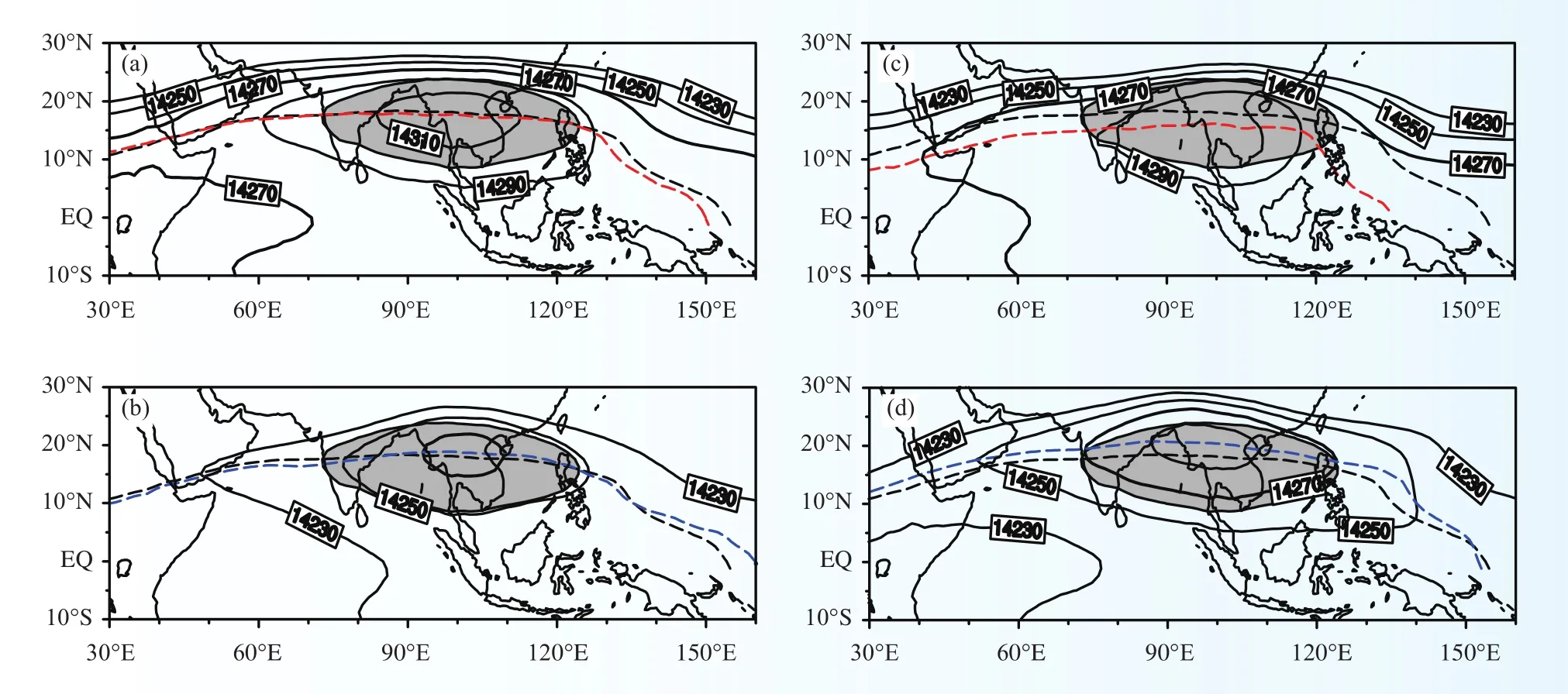
图1 基于南亚高压强度模态指数（a，b）和经向位置模态指数（c，d）的5月150 hPa位势高度合成场（gpm，黑色粗实线和阴影分别表示合成和气候平均14270 gpm等高线，黑色虚线表示气候平均高压脊线，红色和蓝色虚线分别表示强度模态偏强和偏弱时的高压脊线位置）Fig.1 Composites of 150 hPa geopotential height (solid contours, gpm) and ridgeline (dashed curves) of the South Asian High(SAH) with respect to (a, b) the intensity and (c, d) meridional position mode of the SAH on the interannual timescale.The bold solid contours are the 14,270 gpm geopotential height.The climatological 14,270 gpm geopotential height and SAH ridgeline are represented by gray shading and the black dashed curves, respectively

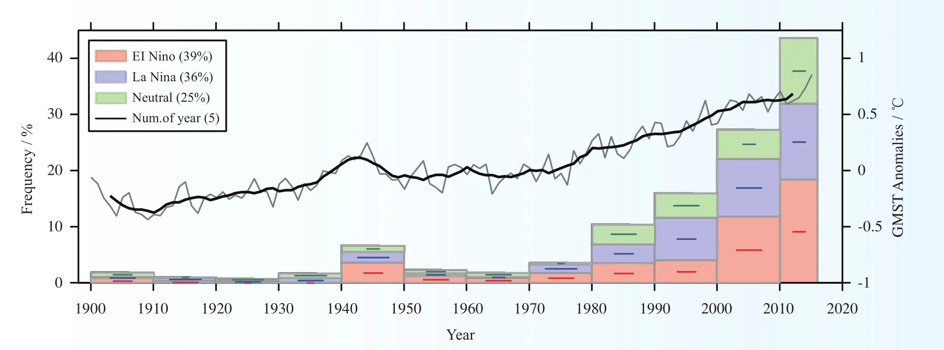
图2 排名前十的年平均高温记录的发生频次（NT10）在各年代的分布(每个年代的El Niño、La Niña和正常年份期间的NT10由不同颜色表示；细线为年平均GMST时间序列，粗线为其7年滑动平均)Fig.2 Relative frequency of the top 10 record (NT10) of annual mean temperatures for each decade.The NT10 is divided into three subgroups (El Niño, La Niña, and neutral years) as indicated as the legend.The NT10 frequency in the 2010s is weighted by 10/6.The number of El Niño, La Niña, and neutral conditions during a decade is indicated by the thick line in each bar.The annual mean GMST is plotted in thin black, and its seven-year moving average is plotted in thick black

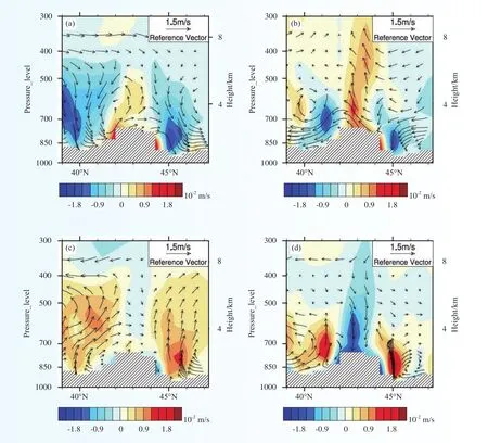
图3 垂直纵剖面的异常垂直运动(颜色阴影；10-2 m/s)及相应的垂直环流(经向风分量和垂直速度的100倍，m/s)在86º和87.5ºE经向平均值：(a)12∶00;(b)18∶00;(c)00∶00;(d)06∶00Fig.3 Vertical profile of the anomalous vertical motion (color shading; 10-2 m s-1) and the corresponding vertical circulation(Vectors having components of the meridional wind and 100 the vertical velocity; m s-1) longitudinally averaged between 86º E and 87.5º E at different times: (a) 12:00; (b) 18:00; (c) 00:00; (d) 06:00

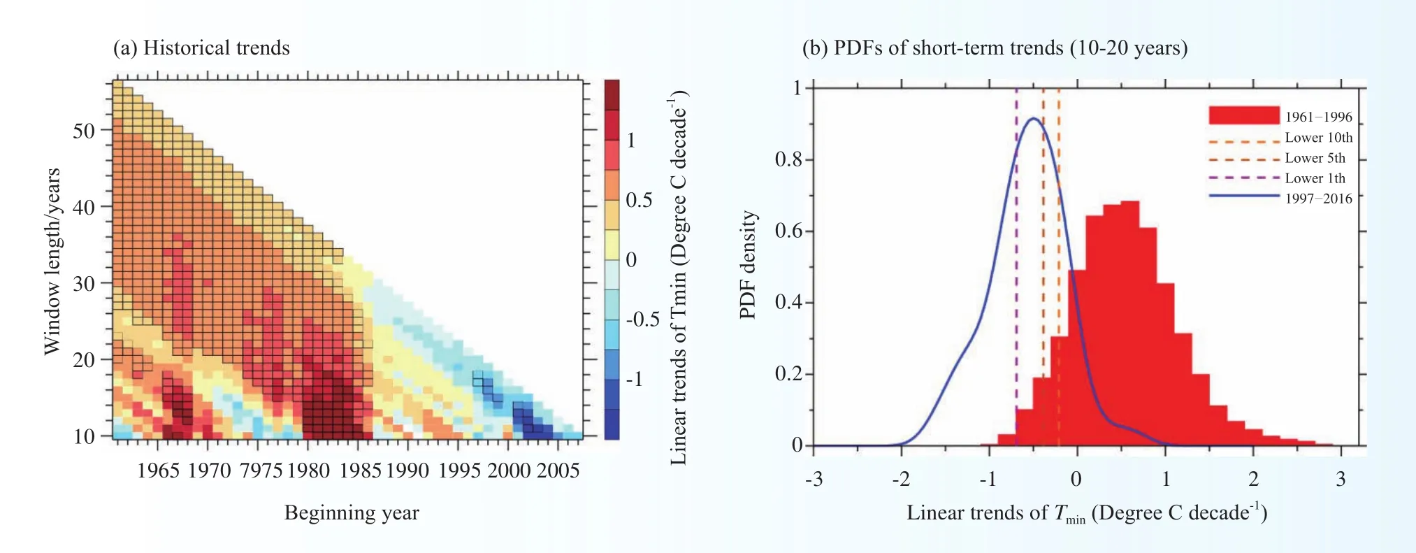
图4 （a）不同起始年份的区域平均最低温度的趋势（℃/10a）和(b)所有短期（10～20年）线性趋势的概率密度函数（图a中黑色正方形表明该趋势至少在0.1的水平上显著；图b中红色梯形为起始年份在1996年以前的线性趋势的概率分布，蓝色线为起始年份在1997年以后的线性趋势的概率分布，3条垂直的虚线为所有早期（开始于1996年以前）的短期趋势中的第10百分位，第5百分位和第1百分位）Fig.4 (a) Historical trends (℃ decade−1) for domain-averaged minimum temperature (Tmin) with different starting years and interval lengths.All trends significant at the 90% conf i dence level at least are enclosed by black squares.(b) PDFs of all shortterm (10−20 years) trends, which began before 1996 (red histograms) and after 1997 (blue curves).Three vertical dashed lines locate the lower 10th, 5th and 1st percentiles of all short-term trends during earlier period (starting before 1996)

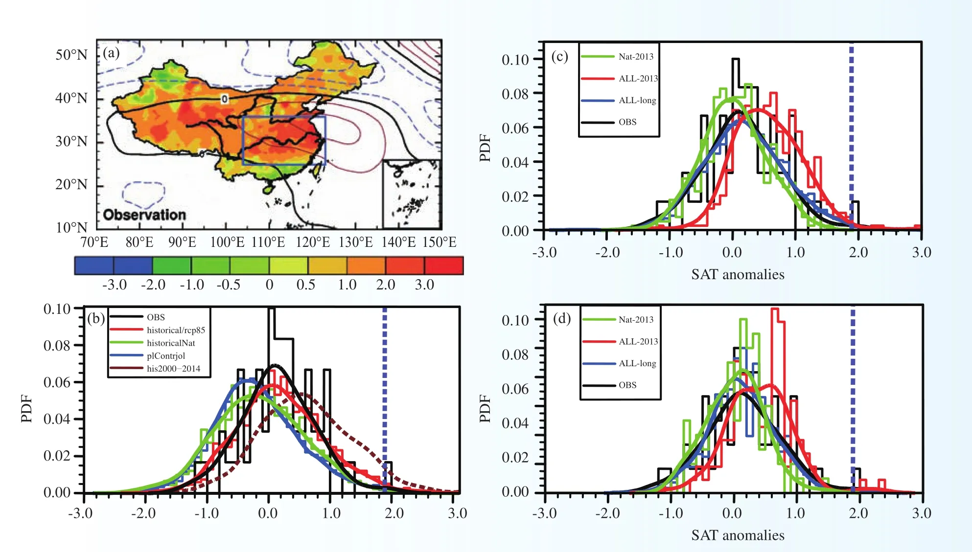
图5 2013年盛夏地表气温（SAT，℃，填色） 和500 hPa位势高度异常（Z500, m，等值线）空间分布(a)； CMIP5(b)、CAM5.1(c)和MIROC5(d)模式模拟的中国中东部盛夏平均SAT异常的直方图（柱状图）和PDF（曲线）（b～d中的紫色线对应2013年盛夏中国中东部SAT异常的观测值）Fig.5 (a) 2013 July–August mean surface air temperature (SAT) anomalies (℃, shaded) and geopotential height anomalies at 500 hPa (Z500, units in m, contours).Histogram (bars) and probability density functions (PDFs, curves) of July–August mean SAT anomalies averaged over Central and Eastern China derived from (b) CMIP5, (c) CAM5.1 and (d) MIROC5 simulations.The vertical purple lines in (b)–(d) are the observed 2013 July–August SAT anomaly

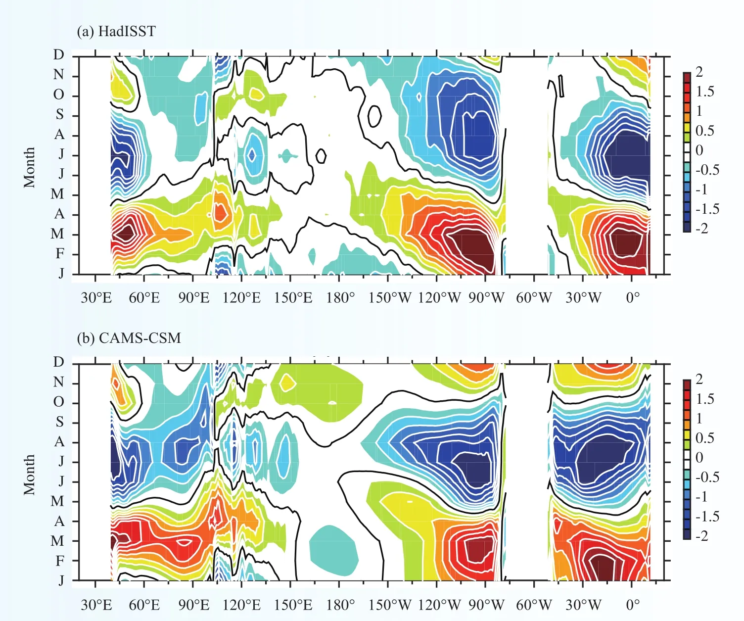
图6 HadISST（a）和CAMS-CSM(b)历史模拟的赤道海温（℃，5°S～5°N平均）气候平均年循环Fig.6 Annual cycle of equatorial SST (℃, averaged over 5°S−5°N) from (a) HadISST and (b) CAMS-CSM historical simulation

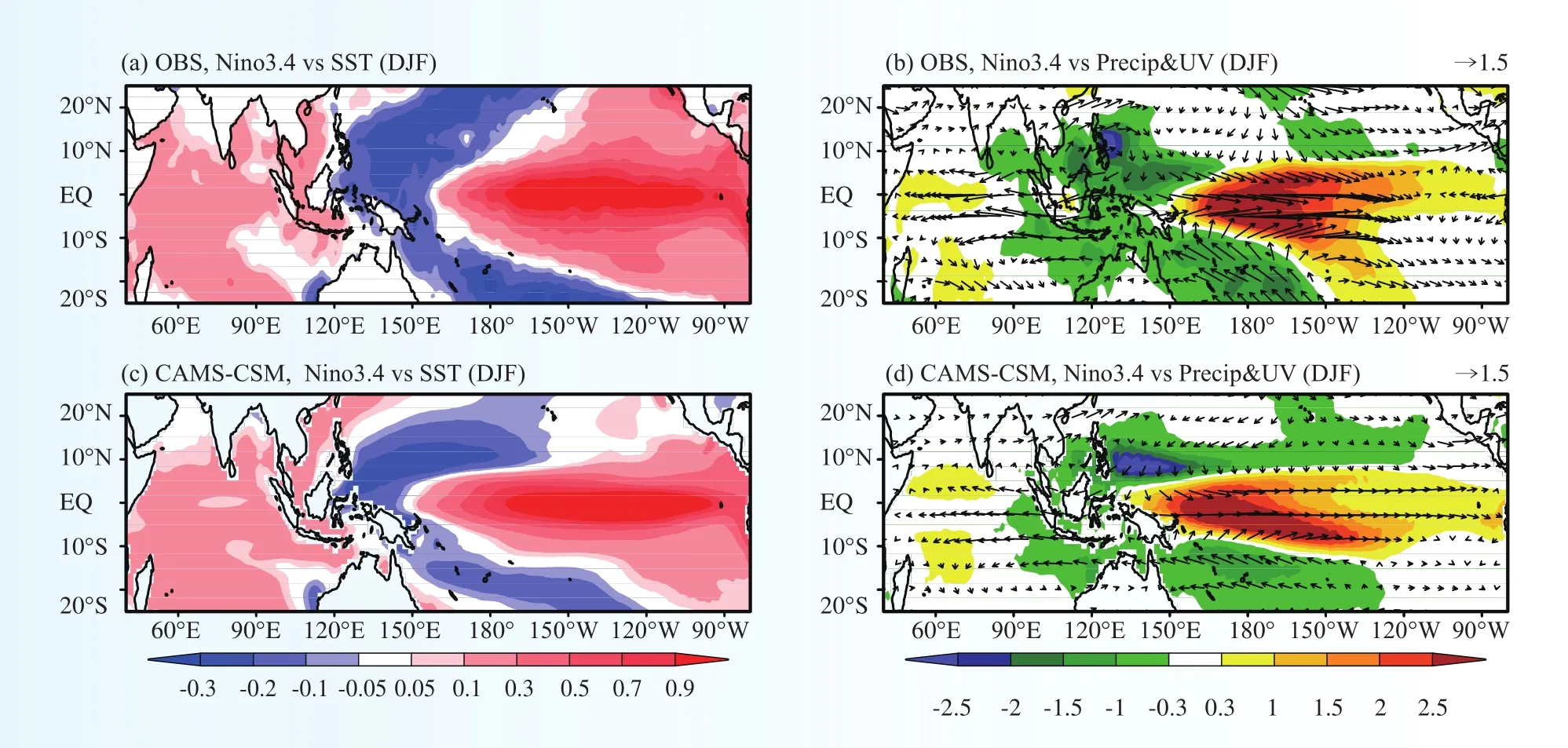
图7 与Nino3.4指数回归所得的冬季(DJF)平均的SST(℃，左图)和降水(阴影，mm /d)和850 hPa风异常(向量，m/s)(右图)(上图为观察结果，下图为CAMS-CSM历史试验模拟结果，其中SST、降水和850 hPa风场分别来自于HadISST、GPCP和NCEP2数据(1980-2013))Fig.7 Winter (DJF) SST (℃, left panels), precipitation (shaded, mm day−1) and 850 hPa winds anomalies (vector, m/s) (right panels) regressed on the Nino-3.4 index from observation (upper panels) and CAMS-CSM piControl simulation (bottom panels).The SST, precipitation and 850 hPa observations are derived from the HadISST, GPCP and NCEP2 data (1980−2013),respectively

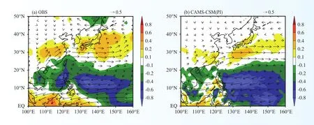
图8 由负WFI指数回归所得夏季降水(阴影，mm/d)和850 hPa风异常(矢量，m/s)：(a)为观测结果；(b)为CAMS-CSM历史试验模拟结果Fig.8 Summer precipitation(shaded, mm/day) and 850 hPa winds anomalies (vector, m s-1) regressed on the negative WFI index from (a) observation and (b) CAMS-CSM (PI) Control simulation

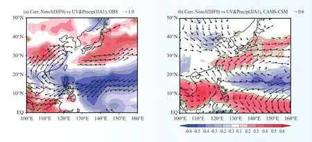
图9 冬季Nino3指数(DJF0)与次年夏季(JJA1)降水(阴影，mm/d)和850 hPa风(矢，m/s)异常的相关系数场：(a)为观测结果；(b)为CAMS-CSM历史试验模拟结果（显示超过95%的信度水平）Fig.9 Correlation between the winter Nino3 index (DJF0) and the following summer (JJA1) precipitation (shaded, mm/day)and 850 hPa wind (vector, m s−1) anomalies from (a) observationand (b) CAMS-CSM (PI) Control simulation.Conf i dence levels above 95% are shown

Progress in Climate System and Climate Change Research

1 Theory and methodology of climate prediction

1.1 Dominant modes of the South Asian High and their mechanism

We have found that two dominant modes exist in the interannual variation of the South Asian High(SAH) in May, in terms of its intensity and meridional position mode, respectively.Both of them are affected by the preceding ENSO events.The pattern variation of SAH in May integrates all onset processes of the Asian summer monsoon as a whole.We have objectively defined the indices of the SAH intensity, western and eastern extension and its meridional position.Two dominant modes were extracted using the principle component analysis (PCA) on the above SAH indices.One is the SAH intensity mode, which presents the uniform variation of the SAH strength and zonal expansion.The other is the SAH meridional position mode featured by the interannual changes of the SAH meridional position with little variation of the SAH intensity.

Although these two modes are affected by the preceding ENSO events, the physical mechanisms are distinct.In boreal spring, the ENSO event is decaying, but its influences on the atmospheric circulation can be memorized by the SSTA in the tropical Indian Ocean (TIO) via the “atmospheric bridge”.Both observation and numerical sensitivity experiments suggest that the relative contribution of SSTA in the tropical Pacific and TIO to the two modes depends on the decaying rate of ENSO event in boreal spring.On the one hand, when the ENSO damps faster, its resultant TIO SSTA can alter the tropical convection over South Asia to modify the SAH intensity mode by stimulating a Rossby wave response over the southwestern India.On the other hand, the SAH meridional position mode is regulated by the SSTA in the tropical Pacific when the ENSO event persists in boreal spring.In particular, the zonal SSTA gradient in the Indo-Pacific Ocean modulates the vertical motion over South Asia, leading to the variation of the meridional temperature gradient in situ.The present study indicates that the interannual variation of the SAH not only depends on the ENSO phase, but also on its temporal evolution in boreal spring (Fig.1).(Liu Boqi, Zhu Congwen)

1.2 Reason for the weaker WPSH in boreal late summer after the 2015/2016 super El Niño.

Previous studies have proposed that the summer WPSH should be enhanced after an El Niño event occurred in the preceding winter.This is partly due to the air-sea interaction over the western North Pacific(WNP), and partly associated with the warming SSTA in the tropical Indian Ocean (TIO) under the influences of El Niño.However, the latest observational studies indicate that the WPSH became weaker in late summer of 2016 after the 2015/2016 super El Niño, which contradicts the existing conceptual model.Compared with the situation in 1983 and 1998, both data analysis and numerical experiment showed that the contrast is primarily attributed to the much faster decaying of the first super El Niño in the 21st century.The fast-decaying El Niño prevented the warming of the TIO in the subsequent summer, which attenuated the anomalous zonal circulation originating from the TIO.Thus, the descending anomaly over the WNP weakened, corresponding to the weaker WPSH.In the meantime, TIO SSTA can alter the mid-latitudinal wave guide in the upper troposphere by changing the meridional temperature gradient.The colder SSTA in the TIO facilitated the southward intrusion of the upper-level wave train into the WNP, which further weakened the WPSH in late summer of 2016.(Liu Boqi, Zhu Congwen, Su Jingzhi, Hua Lijuan)

1.3 Consecutive record-breaking high temperatures marked the handover from hiatus to accelerated warming

Following the recent warming hiatus period, two astonishing high temperature records reached in 2014 and 2015 consecutively.To investigate the occurrence features of record-breaking high temperatures in recent years, a new index focusing the frequency of the top 10 high annual mean temperatures was defined in this study.Analyses based on this index showed that record-breaking high temperatures occurred over most regions of the globe with a salient increasing trend after 1960s, even during the so-called hiatus period.Overlapped on the ongoing background warming trend and the interdecadal climate variabilities, the El Niño events,particularly the strong ones, can make a significant contribution to the occurrence of high temperatures on interannual timescale.High temperatures associated with El Niño events mainly occurred during the winter.As the Pacific Decadal Oscillation (PDO) struggled back to its positive phase since 2014, the global warming returned back to a new accelerated warming period, marked by the record-breaking high temperatures in 2014.Intensified by the super strong El Niño, successive high records occurred in 2015 and 2016 also.Higher frequencies of high temperatures would occur in the near future because the PDO tends to maintain a continuously positive phase (Fig.2).(Su Jingzhi)

1.4 Diurnal variation of summer precipitation across the central Tian Shan Mountains

The climatic features of the diurnally varying summer precipitation over and around the central Tian Shan Mountains are investigated.Both the hourly rainfall data observed at eight stations along a transect across the mountains and the convective index derived from the satellite data show that there are three distinct regimes:the early morning peak at stations to the south of the mountains, the late afternoon peak at stations over the mountains, and the night peak at stations to the north of the mountains.The relationship between regimes of the diurnal variation was analyzed.By defining the regional rainfall event (RRE), the initial stations of each RRE were recorded.The early morning rainfall in the southern periphery of the mountains is triggered locally in the southern basin.Both the late afternoon peak over the mountains and the night peak in the northern periphery are influenced by mountain-originated rainfall events.These rainfall events appear over the mountains in the afternoon, and some of them move northward and lead to the nocturnal rainfall in the northern basin.The triggering of convection in the afternoon over the mountains and that in the early morning in the southern basin are related to the diurnally varying wind and thermodynamic conditions over and around the mountains.Lowlevel convergence with thermodynamic instability appears at noon (night) over the mountains (in the southern basin) just before the start of convection (Fig.3).(Li Jian)

1.5 Genesis of southwest vortices and its relation to Tibetan Plateau vortices

Southwest vortices (SWVs) at 700 hPa occurring over the eastern flanks of the Tibetan Plateau are important summer rain-producing systems, often leading to heavy rainfall over southwestern China and even wider areas in eastern China when they move eastward.Tibetan Plateau vortices (TPVs) are the mesoscale systems forming over the Tibetan Plateau defined at 500 hPa, which have an important influence on SWVs when they move off the Tibetan Plateau.However, only a few studies discussed the effects of TPVs on the genesis of SWVs.The present work compares three situations including 9 cases, using reanalysis data to investigate the role played by TPVs in the genesis process of SWVs.The genesis mechanisms of SWVs accompanied by the moving-off TPVs (Situation A) are explored, and then the mechanisms are further verified by comparison with situations of moving-off TPVs that are unaccompanied by the generation of SWVs(Situation B) and genesis process of SWVs without the moving-off TPVs (Situation C).It is revealed that the TPVs moving-off the Tibetan Plateau (moving-off TPVs) can exert significant effects on the genesis of SWVs through both dynamical and thermodynamic processes.The moving-off TPVs are favorable for the generation of SWVs through strengthening the cyclonic vorticity, convergence and ascending motion.Diagnoses of the potential vorticity budgets reveal that the condensational latent heat has the greatest contribution to the generation of SWVs.The SWVs under the influence of TPVs (Situation A) are stronger and have longer lifespans.Analysis of the water vapor budget indicates that the water vapor is mainly transported from south of the genesis region of SWVs associated with strong southerlies.It is demonstrated that the southerlies and the associated water vapor transport are another prominent factor affecting the genesis of the SWVs.(Li Lun)

1.6 Revisiting summertime hot extremes in China during 1961−2015

Summertime hot extremes in China are categorized into three distinct types, i.e.independent hot days,independent hot nights, and compound events, based on differing configurations between daily maximum and minimum temperatures.Linear trends for multiple indictors of these subtypes and traditionally-defined hot days/nights exhibited remarkable differences in significance, magnitude, and even sign, especially for events involving daytime extremes.Thus, some significant changes masked in conventional analyses are successfully uncovered.Particularly, the dominance of independent hot days has decayed significantly, accompanied by a rapid boom of compound events and/or independent hot nights in different regions.These nighttimeaccentuated hot extremes have exhibited significant increases in duration, intensity and spatial extent, with much stronger trends detected in severest events.(Chen Yang, Zhai Panmao)

1.7 Persisting and strong warming hiatus over eastern China during the past two decades

During the past two decades since 1997, eastern China has experienced a warming hiatus punctuated by significant cooling in minimum temperature (Tmin), particularly during early-mid winter.By arbitrarily configuring start and end years, a “vantage hiatus period” in eastern China is detected over 1998-2013, during which the domain-averagedTminexhibited the strongest cooling trend and the number of significant cooling stations peaked.Regions most susceptible to the warming hiatus are located in North China, the Yangtze-Huai River Valley and South China, where significant cooling inTminpersisted through 2016.This sustained warming hiatus gave rise to increasingly frequent and severe cold extremes there.Concerning its prolonged persistency and great cooling rate, the recent warming hiatus over eastern China deviates greatly from most historical short-term trends during the past five decades, and thus could be viewed as an outlier against the prevalent warming context (Fig.4).(Chen Yang, Zhai Panmao)

1.8 Attribution of the July−August 2013 heat event in Central and East China to anthropogenic greenhouse gas emissions

The observed and simulated frequency, intensity, and duration of some extreme weather and climate events have changed as the climate system has been warming.Extreme event attribution has drawn the interest of the public and been a topic of climate change research because of their severely devastating impacts.An individual extreme weather or climate event can occur because of natural internal variability, and can also be influenced by anthropogenic factors, along with the rare sample of extreme events.Therefore, it’s difficult to determine the extent to which climate change influences individual extreme events.In the midsummer of 2013, Central and East China (CEC) was hit by an extraordinary heat event, with the region experiencing the warmest July–August on record.To explore how human-induced greenhouse gas emissions and natural internal variability contributed to this heat event, we compared observed July–August mean surface air temperature (SAT) with that simulated by climate models.It is found that both atmospheric natural variability and anthropogenic factors contributed to this heat event.This extreme warm midsummer was associated with a positive high-pressure anomaly that was closely related to the stochastic behavior of the atmospheric circulation.Diagnosis of CMIP5 models and large ensembles of two atmospheric models indicates that the human influence has substantially increased the chance of the extreme warm midsummers such as that in 2013 in CEC, although the exact estimated increase depends on the selection of climate models (Fig.5).(Ma Shuangmei)

2 Development of the climate system model

2.1 CAMS-CSM Model description

A new coupled climate model has been developed at the Chinese Academy of Meteorological Sciences(CAMS-CSM) by employing several start-of-the-art component models.The coupled model consists of the atmospheric model ECHAM5, the ocean model MOM4, the sea ice model SIS, the land surface model CoLM,as well as the FMS coupler.The atmospheric component is a modified version of the atmospheric general circulation model ECHAM5 (v5.4) developed at the Max-Planck-Institute for Meteorology (MPI-Met).ECHAM5 is a spectral atmospheric model with a triangular truncation.The major differences between the CAMS-CSM version and the standard ECHAM5 model include: (1) A Two-step Shape Preserving Advection Scheme (TSPAS) is used for the passive tracer transport, which has been shown the capability of reducing the overestimation of precipitation over the steep edges of the southern Tibetan Plateau; (2) A k-distribution scheme developed by Zhang et al.(2006a, 2006b) is adopted for shortwave and longwave radiation transfer calculations.The Tiedtke (1989) massflux scheme with modifications for penetrative convection according to Nordeng (1994) is applied for cumulus convection parameterization.For stability considerations, time-stepping of vertical diffusion is treated implicitly in the ECHAM5 model.The implicit algorithm results in a tridiagonal system for momentum, temperature and water vapor tendency, in which the surface fluxes are relying on the states of next time step and thus can only be obtained after solving the tridiagonal equations in the atmospheric model.The model exhibits capability of reproducing the climatological mean states and seasonal cycle of major quantities of the climate system, including sea surface temperature, precipitation, sea ice extent, as well as thermocline.The major modes of climate variability are also reasonably captured by the model, such as the Madden-Julian Oscillation (MJO), ENSO, the East Asian Summer Monsoon (EASM), as well as the Pacific Decadal Oscillation (PDO).In particular, the model displays promising advantage in simulating the East Asian Summer Monsoon (EASM) variability and the ENSO-EASM relationship.Several biases exist in the model:the double-ITCZ in the annual mean precipitation map, overestimated ENSO amplitude, and too weaker Bjerkness feedback associated with ENSO.

2.2 Precipitation

Overall, the general spatial pattern of the annual mean precipitation in the model resembles that from the observations.The major rainfall center, such as ITCZ, SPCZ, and those over the tropical Indian Ocean as well as the tropical Atlantic are clearly seen in the model.The major rainbelts, as well as the seasonal migration of the intertropical convergence zone (ITCZ) and the south Pacific convergence zone (SPCZ) are reasonably captured by the model.The simulated ITCZ moves to its northernmost position with precipitation peak in July–August., while SPCZ is strongest and at its southernmost position in February–March., in good agreement with observations.During May to December., the ITCZ dominates precipitation over the tropical region, while the SPCZ is prevailing from January to April, such a seasonal timing feature is consistent between the model simulation and observations.

2.3 SST seasonal cycle and thermocline

ENSO is the most dominant climate mode on interannual time scales in the climate system.Evident anomalies of the atmosphere and ocean have been observed during the ENSO cycles, including SST,precipitation, zonal wind, as well as the thermocline.The change in thermocline depth can lead to fluctuation in SST in the eastern equatorial Pacific by upwelling and mixing, referred as the thermocline feedback, playing an important role in ENSO dynamics.The thermocline feedback is most effective in the central-eastern equatorial Pacific because of the shallow thermocline there.Therefore, realistically representing the mean thermocline and its seasonal cycle is crucial for the simulation of ENSO.Compared with the observation, the thermocline depth is well reproduced by the model.The simulated thermocline is somewhat deeper in the western Pacific and shallower in the eastern Pacific, indicating a slightly stronger zonal slope of thermocline in the model simulation.A distinctive feature of ENSO is its phase-locking to winter.Previous studies proposed that the seasonal variations of climatological states are crucial for the ENSO phase-locking.One of the essential metrics to measure the seasonal variation of tropical climatology is the seasonal cycle of the equatorial SST.Qualitatively, the model does a good job in reproducing the observed seasonal cycle of equatorial SST.The annual-cycle in the eastern equatorial Pacific as well as the semi-annual-cycle in the western equatorial Pacific are captured by the model.There are some discrepancies in the model, primarily occurring in the eastern Pacific.First, the simulated magnitude of the warm phase is weaker than the observed values, whereas that of the cold phase is stronger.Second, the cold phase in the model tends to peak earlier than that in observation by 1–2 months (Fig.6).

2.4 ENSO

The regression pattern between the Nino3.4 index and SST anomalies in the tropical Pacific and Indian Ocean are shown in Figs.7a and 7c.Overall, the anomalous SST pattern during El Niño events is reasonably captured by the model.Compared with the HadISST SST data, the simulated positive SSTA over the central and eastern Pacific is too narrow in the meridional direction and extends more westward as a result of the excessive westward penetration of the cold tongue in the model.The negative anomalies in the western Pacific exhibit a much zonal orientation on the north lobe, while on the south lobe the strength appears to be weaker than that in observations.The spatial pattern and magnitude of the warm signal over the South China Sea and tropical Indian Ocean are successfully simulated, as well as the small negative area on the west coast of Australia.The regression between Nino3.4 index and precipitation and 850 hPa wind anomalies are further shown in Figs.7b and 7d.The anomalous pattern is characterized by the increased precipitation over the central equatorial Pacific as a result of the enhanced convection in response to the warm SSTA.Meanwhile, anomalous westerlies extend from 150°E to 120°W over the equatorial Pacific Ocean, indicating the atmospheric aspect of the Bjerkness feedback.Negative precipitation anomalies spread over the eastern Indian Ocean and the regions of cold SSTAs, due to the weakened Walker circulation and suppressed convection over there.The model shows its ability to capture the spatial pattern of precipitation and wind anomalies associated with ENSO.The anomalous precipitation centers and low-level winds in both Pacific and Indian Oceans are reproduced with comparable magnitudes relative to those in observations.For example, the model captures the observed asymmetrical feature of precipitation and low-level wind anomalies: both precipitation and low-level wind anomalies tend to maximize south of equator.

2.5 East Asian summer monsoon (EASM) variability

As precipitation and winds are usually used to represent the EASM, in this study the evaluation mainly focused on the precipitation and wind variations associated with the EASM variability.While a number of indices have been proposed to measure the strength of the EASM (Wang 2008), here the monsoon index by Wang and Fan (1999) is adopted, which is defined as the 850 hPa zonal wind shear: WFI=U850(5°−15°N,90°−130°E) −U850(22.5°−32.5°N, 110°−140°E).

Fig.8 shows the regression pattern between the negative WFI and the 850 hPa wind and precipitation anomalies from observations and the model.The observed circulation pattern is characterized by an anticyclone with anomalous southwesterly winds over southeastern China and westerly along the Yangtze River (YRV)and the southeast of Japan, as well as the increased easterly stretching from the western Pacific to the South China Sea.The precipitation pattern displays enhanced rainbelt spanning along the East Asian subtropical front and suppressed rainfall spreading in the southern wing of the anticyclone, with the anomalous precipitation centers close to the climatological rainfall centers.Overall, the model does a fairly good job in reproducing the observed pattern.The enhanced/deficit rainbelt over the northern/southern wing of the anticyclone is captured by the model.In particular, the model is able to capture the anomalous rainfall centers associated with the variations of Meiyu/Baiu/Changma rainbelt, which remains poorly simulated by most of the present-day climate models.

The distribution of winds and precipitation in Fig.8 reflects the anomalous pattern during the decaying summer of El Niño event, which also features an anticyclone over the northwestern Pacific and appears to be the dominant mode of the EASM interannual variability.This anticyclone, referred to as the western North Pacific anticyclone (WNPAC), originates in the autumn of the developing phase and sustains to the decaying summer of El Niño event, providing a mechanism connecting the summer precipitation of China and ENSO.While the mechanism of sustaining the WNPAC through the decayed summer is controversial, it might link to the combined forcing from northwestern Pacific, the Indian Ocean, as well as the tropical North Atlantic Ocean.To examine how well the model captures this dominant pattern in the ENSO-EASM relationship,the correlation between winter Niño3 index and the following summer precipitation and 850 hPa wind anomalies are calculated with the results shown in Fig.9.Indeed, the correlation pattern resembles that in Fig.8, suggesting that the dominant mode of the EASM is closely related to ENSO.The model successfully reproduces the ENSO related pattern for both precipitation and 850 hPa wind anomalies.The anomalous anticyclonic circulation over the WNP can be clearly observed from the simulated pattern.Analogous to that in the GPCP data, the simulated anomalous Meiyu/Baiu/Changma rainbelt stretches from the eastern China to the southeast of Japan, suggesting that the model has a fairly good capability in simulating the ENSO-EASM relationship.(Rong Xinyao, Li Jian, Chen Haoming, Xin Yufei, Su Jingzhi, Hua Lijuan, Qi Yanjun, et al.)

3 Polar research

3.1 Snowdrift effect on snow deposition: Insights from a comparison of a snow pit profile and meteorological observations in east Antarctica

A high-frequency, precise ultrasonic sounder was used to monitor precipitated/deposited and drift snow events over a 3-year period (17 January 2005 to 4 January 2008) at the Eagle automatic weather station site,inland Antarctica.Ion species and oxygen isotope ratios were also generated from a snow pit below the sensor.These accumulation and snowdrift events were used to examine the synchronism with seasonal variations of δ18O and ion species, providing an opportunity to assess the snowdrift effect under typical Antarctic inland conditions.There were up to 1-year differences for this 3-year-long snow pit between the traditional dating method and ultrasonic records.This difference implies that in areas with low accumulation or high wind, the snowdrift effect can induce abnormal disturbances on snow deposition.The snowdrift effect should be seriously taken into account for high-resolution dating of ice cores and estimation of surface mass balance, especially when the morphology of most Antarctic inland areas is similar to that of the Eagle site.(Ding Minghu)

3.2 A comparison of two Stokes ice sheet models applied to the Marine Ice Sheet Model Intercomparison Project for plan view models (MISMIP3D)

We presented a comparison of the numerical and simulation results for two “full” Stokes ice sheet models,FELIX-S and Elmer/Ice.The models were applied to the Marine Ice Sheet Model Intercomparison Project for plan view models (MISMIP3D).For the diagnostic experiment (P75D) the two models gave similar results (with＜ 2% difference in terms of along-flow velocities) when using identical geometries and computational meshes,which we interpreted as an indication of inherent consistencies and similarities between the two models.For the standard (Stnd), P75S, and P75R prognostic experiments, we found that FELIX-S (Elmer/Ice) grounding lines were relatively more retreated (advanced) with the results that were consistent with minor differences in the diagnostic experiment results.We showed that this is due to different choices in the implementation of basal boundary conditions in the two models.While we were unable to argue for the relative favorability of either implementation, we did show that these differences decreased with increasing horizontal (i.e., both along- and across-flow) grid resolution and that grounding-line positions for FELIX-S and Elmer/Ice converged within the estimated truncation error for Elmer/Ice.Stokes model solutions are often treated as an accuracy metric in model intercomparison experiments, but computational cost may not always allow for the use of model resolution within the regime of asymptotic convergence.In this case, we proposed that an alternative estimate for the uncertainty in the grounding-line position is the span of grounding-line positions predicted by multiple Stokes models.(Zhang Tong)

3.3 Comparison of long-term total ozone observations from space- and ground-based methods at Zhongshan Station, Antarctica

Total ozone errors for satellite observations at Zhongshan Station in Antarctica were characterized using their relative difference (RD) from ground-based Brewer observations during 1993–2015.All satellite total ozone observations slightly overestimated ground-based ones (with RD less than 4%).This is in contrast to the conclusions drawn from global-scale validation studies, where main ground-based reference stations are located in middle latitudes.Given multiple total ozone data per day at Zhongshan Station, observed by a sun synchronous orbit satellite, measurements at the lowest solar zenith angle (SZA) showed greatest consistency with Brewer ones, having an overall RD of −0.02%–1.15%.Algorithm-retrieved total ozone data from the total ozone mapping spectrometer (TOMS), including solar backscatter ultra violet (SBUV), TOMS-Earth probe (EP), ozone monitoring instrument (OMI)-TOMS, showed the best agreement with ground-based values,followed by the global ozone measurement experiment-type direct fi tting (GOD-FIT) algorithm for the GOME-2A, and finally the differential optical absorption spectroscopy (DOAS) —Algorithm retrieved products for satellites-detectors of global ozone measurement experiment (GOME), scanning imaging absorption spectrometr for atmospheric chartography (SCIAMACHY), and OMI.Satellite total ozone RD presented some statistical characteristics, but no specific trends.Values for DOAS and GOME-2A algorithms significantly increase when the SZA was above 60°–70°, whereas values for GOME-2A decrease when the SZA is 80°–85°.Satellite total ozone RD is the minimum when the Brewer total ozone is 300–350 DU, with an obvious increase in RD values for DOAS- and GOME-2A when the Brewer total ozone is 150–300 DU.Satellite total ozone RD obviously increases as the time difference between satellite overpasses and Brewer measurements grows.Specifically, RD rises as the absolute time difference increases to more than 4 h, yielding an OMI-TOMS RD of more than 10% as this difference increases to 8 h.The DOAS- RD may be up to 15%, while GOME-2A RD does not exceed 10%.The satellite total ozone RD may reach −5%, as the distance between the satellite overpass pixel and the station become more than 100 km.Possibly because of the discrepancy in surface albedo, the TOMS-algorithm retrieved total ozone is underestimated when the pixel on the south-east side of the station (the Antarctica continent) is used but overestimated on the north-west side of the station (the Indian Ocean).Consistency between space- and ground-based total ozone data is least for the “ozone hole”.Typically,the RD of TOMS-algorithm retrieved total ozone is within 1%/10yr.Thus, the SBUV and Brewer monthly averaged total ozone anomalies from 1996 to 2015 were 1%/10yr and 0.9%/10yr, respectively.Both indicate a weak but consistent ozone layer recovery.(Zhang Lei)

3.4 Significant increase of the Antarctic sea ice extent in the Ross Sea

In the context of global warming, the question of why Antarctic sea ice extent (SIE) has increased is one of the most fundamental unsolved mysteries.Although many mechanisms have been proposed, it is still unclear whether the increasing trend is anthropogenically originated or only caused by internal natural variability.In this study, we employed a new method where the underlying natural persistence in the Antarctic SIE can be correctly accounted for.It is found that the Antarctic SIE is not simply short-term persistent as assumed in the standard significance analysis, but actually characterized by a combination of both short- and long-term persistence.By generating surrogate data with the same persistence properties, the SIE trends over Antarctica (as well as five sub-regions) are evaluated using Monte-Carlo simulations.It is found that the SIE trends over most sub-regions of Antarctica are not statistically significant.Only the SIE over Ross Sea has experienced a highly significant increasing trend (p=0.008) which cannot be explained by natural variability.Influenced by the positive SIE trend over Ross Sea, the SIE over the entire Antarctica has also increased over the past decades,but the trend is only marginally significant (p=0.034).(Yuan Naiming, Ding Minghu)

3.5 A cold event in Asia during January−February 2012 and its possible association with Arctic seaice loss

Through both observational analyses and simulation experiments, the intraseasonal evolution of atmospheric circulation anomalies associated with a persistent cold event in the Asian continent during late January to early February 2012, and the possible association with Arctic sea-ice loss were investigated.The results suggest that the northeastern Pacific-Aleutian region and central Eurasia are two critical areas where the atmospheric circulation evolution contributed to the development of this cold event.A persistent increase in sea level pressure (SLP) over the Aleutian region was a predominant feature prior to the cold event, and then decreasing SLP over this region was concurrent with both occurrence of a polar blocking high aloft and the rapid strengthening of the Siberian High, triggering outbreaks of Arctic air over the Asian continent.Consequently, the influence of the Aleutian region on this cold event, i.e., the downstream effect of the atmospheric circulation, played a critical role.Results from simulation experiments demonstrate that Arctic atmospheric circulation conditions in the summer of 2011 significantly enhanced a negative feedback of Arctic sea-ice loss on SLP over the Aleutian region and central Eurasia during the ensuing wintertime, which may be a major reason for the development of this cold event.This finding also implies that the Aleutian Low and disturbances in the mid-latitudes over the northeastern Pacific may provide precursors to increase skills in predicting the intraseasonal evolution of extreme cold events over Eurasia.(Wu Bingyi)

3.6 Winter Olympics services

Since November 2015, according to the two difficulties that guarantee of pistes and the snow storage evaluation in the Winter Olympic Games, the observation of snow was carried out in Chongli and Yanqing,and the preliminary results were obtained in terms of artificial snow evolution and snow and ice monitoring of track.In view of preparing a ski racing track, one of the core issues of the racing track quality, we have initially established a quantif i able scientific solution through the literature research, the Winter Olympic Games Group Committee discussion, the International Snow Union Expert consultation, the field investigation and so on.Combined with oversea experience and meteorological monitoring scheme of snow and ice in polar, the project puts forward the quality monitoring scheme of snow and ice on pistes and carries out the field experiment in Wanlong ski resort in Chongli, which is in progress well.Based on the polar ice-gas interaction model and the Snow Evolution model, a forecast model for the quality of snow and ice on pistes was established, and a running manual was written.

3.7 Polar meteorological service

We have fulfilled meteorological observations at Zhongshan station and Great Wall station in Antarctic.We also have fulfilled ozone observations at Zhongshan station and helped to release “Antarctic Ozone Bulletin”.We have made new progress in Ultralow temperature AWS research and development.We have rebuilt LGB69 and Dome A Ultralow temperature AWS and acquired continuous observational data in 2017.