Zhang Shaolin (张少林), Jing Fengshui, Wang Shuo

(*The State Key Laboratory of Management and Control for Complex Systems, Institute of Automation, Chinese Academy of Sciences, Beijing 100190, P.R.China) (**University of Chinese Academy of Sciences, Beijing 100190, P.R.China)

A transition method based on Bezier curve for trajectory planning in cartesian space①

Zhang Shaolin (张少林)***, Jing Fengshui***, Wang Shuo②

(*The State Key Laboratory of Management and Control for Complex Systems, Institute of Automation, Chinese Academy of Sciences, Beijing 100190, P.R.China) (**University of Chinese Academy of Sciences, Beijing 100190, P.R.China)

In order to smooth the trajectory of a robot and reduce dwell time, a transition curve is introduced between two adjacent curves in three-dimensional space. G2 continuity is guaranteed to transit smoothly. To minimize the amount of calculation, cubic and quartic Bezier curves are both analyzed. Furthermore, the contour curve is characterized by a transition parameter which defines the distance to the corner of the deviation. How to define the transition points for different curves is presented. A general move command interface is defined for receiving the curve limitations and transition parameters. Then, how to calculate the control points of the cubic and quartic Bezier curves is analyzed and given. Different situations are discussed separately, including transition between two lines, transition between a line and a circle, and transition between two circles. Finally, the experiments are carried out on a six degree of freedom (DOF) industrial robot to validate the proposed method. Results of single transition and multiple transitions are presented. The trajectories in the joint space are also analyzed. The results indicate that the method achieves G2 continuity within the transition constraint and has good efficiency and adaptability.

transition method, Bezier curve, G2 continuity, transition constraint

0 Introduction

A robot program consists of several motion commands and each command defines a curve. The most common curves are lines and circles, which are connected head-to-tail in sequence. However, two adjacent curves may be not smooth at the intersection. The robot has to halt at the terminal of a curve to avoid velocity fluctuation. So, it is necessary to introduce a transition part between two curves to smooth the trajectory and reduce the dwell time.

In PLCopen Motion Control Specifications[1,2], the way of connecting two curves without halt is called blending mode. In this mode, a transition curve is inserted between two adjacent curves. In order to transit smoothly, the transition curve needs to satisfy some smoothness criteria. G2 continuity[3]is usually adopted as the criterion. Furthermore, the transition curve should be characterized to adapt to different applications. For example, smoothness is more important for a transportation robot, and accuracy is more important for a welding robot. So, the smoothness and accuracy should be able to be adjusted for different applications.

There are already many investigations about transition curves, especially in the field of transition between lines[4-10]. Sencer, et al.[4]proposed a method to transit between adjacent lines with quintic B-splines. G2 continuity was guaranteed and the cornering tolerance could be set by the user. Bi, et al.[5]utilized cubic Bezier curve to transit between adjacent lines. Also, G2 continuity was guaranteed, and the curvature of the transition curve was analyzed. Zhao, et al.[6]utilized a curvature-continuous B-spline with five control points for transition. Hota, et al.[7]proposed a path namedγ-trajectoryfortransition.Theirstudiesshowedthatvariousmethodscouldbeusedtotransitbetweenlines.Buttheydidnotillustratehowtodeterminetheorderofthetransitioncurve.

Thetransitionincludingcircleshasalsobeeninvestigatedinsomefields[11-14].Habib,etal.[11]describedamethodbasedonasinglecubicBeziercurvetojointwocircles.ThetransitioncurvewasS-shapedorC-shaped,andofG2continuity.Thismethodwasappliedtohighwayandrailwayroutedesign.AsimilarworkwasdonebyAhmadAetal.[12],butquarticBezierspiralwasusedfortransitioninstead.Rashid,etal.[13]proposedanS-shapedtransitioncurvetojointwotangentcirclesofthesamediameter,whichwasusedtodesignaSpurGearTooth.Mostofthestudiesfocusedonplanartransitionindifferentapplications.However,fewstudieshavebeendoneontransitionbetweenadjacentlinesandcircleswithshapecontrol,especiallyinthree-dimensionalspace.

Inthispaper,atransitionmethodisdevelopedbasedonBeziercurvetoachieveG2continuity.Forefficiencyofthealgorithm,asinglecurveisadoptedfortransition.CubicBeziercurveistriedfirstbecauseitisoflowdegreeandeasilycalculated.IfcubicBeziercurvedoesnotmeetthesmoothnessconstraint,quarticBeziercurvewillbeused.Differentsituationsarediscussedseparately,includingtransitionbetweentwolines,transitionbetweenalineandacircleandtransitionbetweentwocircles.Thelinesandcirclesaresupposedtobeinthree-dimensionalspacewithoutanylimitationsforthecircleradii,andthelengthoflineandcircle.Furthermore,tocharacterizethecontourcurve,atransitionparameter(TP)whichdefinesthedistancetothecornerofthedeviationisadopted.Ifarobotismovingalongacurve,thetransitionwillstartwhentheremaininglengthisshorterthanTP.

The remaining part of this paper is organized as follows. Section 1 introduces a general transition interface and a planning procedure. How to transit between two adjacent curves is presented in Section 2. The transition method is demonstrated with experiments in Section 3. Finally, conclusions are given in Section 4.

1 Transition interface and planning procedure

Transition curve is inserted between two adjacent curves and the speed is re-planned, as shown in Fig.1. Transition planning is a part of trajectory planning. Transition planning reads motion commands from program, and prepares the curves for interpolation. For example, there are three move line (MovL) commands in a robot program. The transition interface for program is shown in Fig.2, the desired trajectory is shown in Fig.3, and the general transition planning procedure is shown in Fig.4.

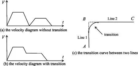
Fig.1 Velocity diagram for transition

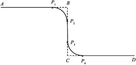
Fig.3 An example of three lines for transition

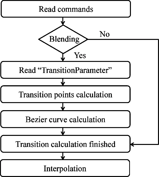
Fig.4 A flow chart for transition planning procedure

Firstly, the transition planning task reads transition commands. If the “TransitionMode” parameter of the MovL (lineAB) command is “blending”, a transition curve will be inserted between lineABand lineBC. TransitionP1P2startsatpointP1andendsatpointP2.ThelengthoflineP1BandlineBP2aredefinedasAlgorithm1.TPABhereisshortfor“TransitionParameter”parameteroftheMovL(lineAB) command. The lengths of lineP3CandlineCP4arecalculatedsimilarly.

IfthelengthoflineABand lineBCare both larger than 2·TPAB,thelengthoflineP1BandlineBP2areequaltoTPAB.Otherwise,theyaredefinedintermsofthelengthoflineABand lineBC. So, lineBCmay have two different transition points or two overlapping points. More examples are shown in Fig.5.

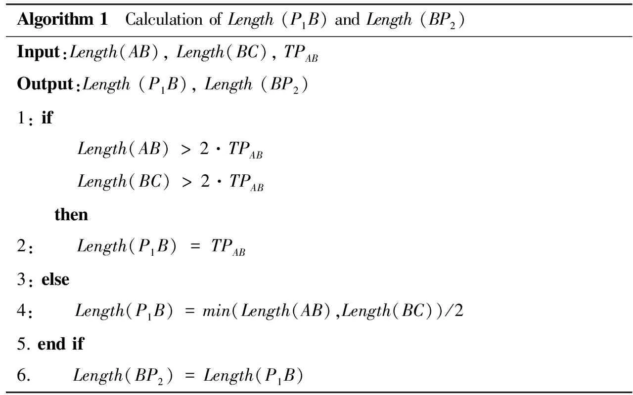
Algorithm1 CalculationofLength(P1B)andLength(BP2)Input：Length(AB)，Length(BC)，TPABOutput：Length(P1B)，Length(BP2)1：if Length(AB)>2·TPAB Length(BC)>2·TPAB then2： Length(P1B)=TPAB3：else4： Length(P1B)=min(Length(AB)，Length(BC))/25．endif6． Length(BP2)=Length(P1B)

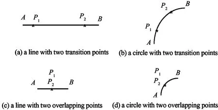
Fig.5 The transition points of lines and circles

After getting the information of the transition points, the transition curve could be calculated, as will be introduced in Section 2. Then, it is ready for interpolation.

2 A transition method based on a single Bezier curve

2.1 Preliminaries

Given spatial control pointsPi(i=0,1,2,…,n),theinterpolationforeachpointontheBeziercurveis

(1)

where

(2)

TheBeziercurveisaweightedaverageofeachcontrolpoint.ItbeginsatP0andendsatPn.TheBeziercurvehastheconvexhullproperty,whichmeansthatthecurvedoesnot“undulate”morethanthepolygonofitscontrolpoints.ForcubicBeziercurve(n=3),fourcontrolpointsareneeded.Forhigher-ordercurves,theamountofcomputationwillbelargerandmoreintermediatepointsareneeded.

ThederivativesforaBeziercurveatC(0)andC(1)are

(3)

Thesecondderivativesare

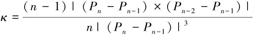
(4)

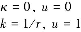
ForG2continuity,theadjacentcurvesshareacommontangentdirectionandacommoncenterofcurvatureatthejoinpoint[3].ThecurvatureatC(0)andC(1)shouldbe

(5)

SubstitutingEq.(3)andEq.(4)intoEq.(5)yields

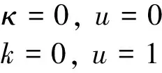
(6)

u=1 (7)

2.2Transitionbetweentwolines

Fig.6showsacaseofacubicBeziercurve(n=3)transitingfromlineABtolineBC.PointP0andpointP3arethetransitionpointssetbyAlgorithm1.

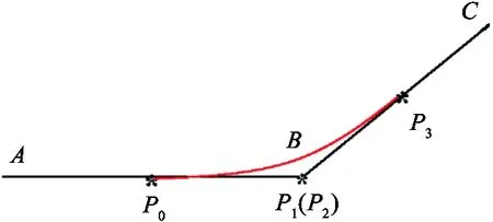
Fig.6 The transition between two lines

1) The transition curve should be tangent with lineABandlineBC.

FromEq.(3),controlpointP1shouldbeonlineAB,andcontrolpointP2shouldbeonlineBC.

(8)

2)ThetransitioncurveshouldhavethesamecurvaturewithlineABand lineBC.

(9)

From Eqs(6)～(9), pointP1andpointP2shouldoverlapatpointB.Then,thetransitionBeziercurveisgivenbypointP0,pointP1,pointP2,andpointP3.

2.3Transitionbetweenalineandacircle

Fig.7showsacaseofacubicBeziercurve(n=3)transitingfromlineABtocircleBC.PointP0andpointP3arethetransitionpointssetbyAlgorithm1.

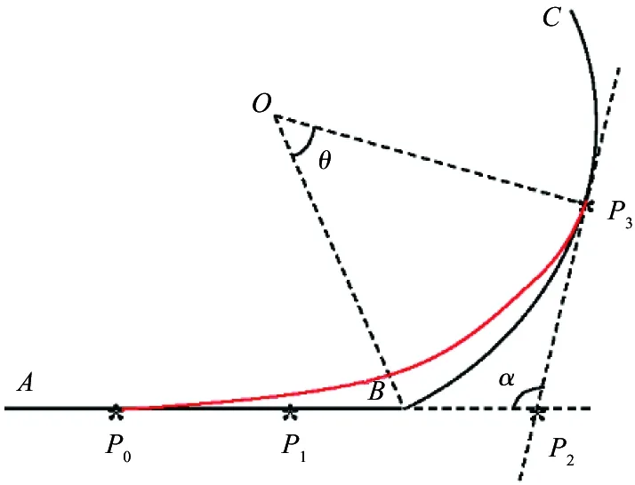
Fig.7 The transition between a line and a circle

1) The transition curve should be tangent with lineABandcircleBC.

FromEq.(3),controlpointP1shouldbeonlineAB,andcontrolpointP2shouldbeonthetangentlineofcircleBCatpointP3.

(10)

(11)

2)ThetransitioncurveshouldhavethesamecurvaturewithlineABandcircleBC.

(12)

whereristheradiusofcircleBC.

FromEqs(6),(7)andEqs(10)～(12),pointP1andpointP2aredefined.IfpointA,pointB,pointCandpointOarecoplanar,thesolutionisgivenasfollows.Otherwise,thereisnosolution.

1)PointP2istheintersectionoflineP0P1andlineP3P2.

2)FromEq.(7)andEq.(12),Eq.(13)isgot.Then,pointP1isgivenbyEq.(10)andEq.(13).

(13)

whereα=∠P1P2P3.

QuarticBeziercurve(n=4)couldmeetthesmoothnessconstraintshere(seeFig.8).PointP0andpointP4arethetransitionpointssetbyAlgorithm1.PointP1,pointP2andpointP3aregivenasfollows:

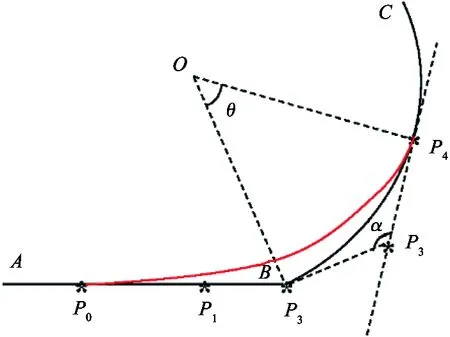
Fig.8 The transition between a line and a circle (quartic Bezier curve)

1) PointP2

Intuitively, in order to track the given trajectory, pointP2shouldbearoundlineABorcircleBC.Forthesimplicityofcalculation,pointP2issetatpointB.

2)PointP3

SimilartoEq.(11),thereexists:

(14)

FromEq.(7)andEq.(12),

(15)

whereα=∠P2P3P4,θ=∠P2OP4, 0<θ<2pi.

FromEq.(14)andEq.(15),pointP3isobtained.

3)PointP1

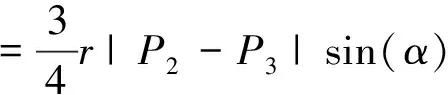
FromEq.(6),Eq.(10)andEq.(12),therearemultiplesolutionsforpointP1.Anoptimizationindexcanbeaddedtoobtaintheoptimalsolution.OneansweristoaddaconstraintasEq.(16).Approximately,εmeansameasureofcurvature.Thustogettheminimumofεmakesthetransitioncurvebendatleast[15].

(16)

Letdε/dl1=0,l1=|P1-P0|.SubstitutingEq.(1)intoEq.(16)yields

(17)

where

FromEq.(10)andEq.(17),pointP1isobtained.

Then,thetransitionBeziercurveisgivenbypointP0,pointP1,pointP2,pointP3andpointP4.

2.4Transitionbetweentwocircles

Fig.9showsacaseofacubicBeziercurve(n=3)transitingfromcircleABtocircleBC.PointP0andpointP3arethetransitionpointssetbyAlgorithm1.

Fig.9 The transition between two circles (cubic Bezier curve)

1) The transition curve should be tangent with circleABandcircleBC.

FromEq.(3),controlpointP1shouldbeonthetangentlineofcircleABatpointP0,andcontrolpointP2shouldbeonthetangentlineofcircleBCatpointP3.

(18)

(19)

2)ThetransitioncurveshouldhavethesamecurvaturewithcircleABandcircleBC.

(20)

wherer1istheradiusofcircleAB,andr2istheradiusofcircleBC.

FromEqs(6),(7)andEqs(18)～(20),pointP1andpointP2aredefined.However,itisdifficulttoobtaintheanalyticalsolutionshere.Numericalmethodcanbeusedtosolvethesefunctions,butwithalargeamountofcomputation.

QuarticBeziercurve(n=4)couldmeetthesmoothnessconstraintshere,seeFig.10.PointP0andpointP4arethetransitionpointssetbyAlgorithm1.PointP1,pointP2andpointP3aregivenasfollows:

Fig.10 The transition between two circles (quartic Bezier curve)

1) PointP2

SimilartoSection2.3,pointP2issetatpointB.

2)PointP3

SimilartoEq.(19),thereexists:

(21)

FromEq.(7)andEq.(20),

(22)

whereα2=∠P2P3P4,θ2=∠P2O2P4, 0<θ2<2pi.

FromEq.(21)andEq.(22),pointP3isobtained.

3)PointP1

SimilartoEq.(21)andEq.(22),thereexist:

(23)

(24)

whereα1=∠P0P1P2,θ1=∠P0O1P2, 0<θ1<2pi.

FromEq.(23)andEq.(24),pointP1isobtained.

Then,thetransitionBeziercurveisgivenbypointP0,pointP1,pointP2,pointP3andpointP4.

Mark 1 Although Figs6～10 illustrate conditions for planning on plane, the transition method is also feasible for spatial planning, as will be shown in Section 3.

3 Experiments

The transition method is evaluated by several experiments on a six DOF robot—ER20-C10. The control system is shown in Fig.11. The original motion controller is replaced by an industrial computer CX5130 made by Beckhoff company. In addition to the transition method, some other components are also realized for the experiment, such as robot program interpreter, trajectory planning method for line and circle commands, and forward and inverse kinematics.

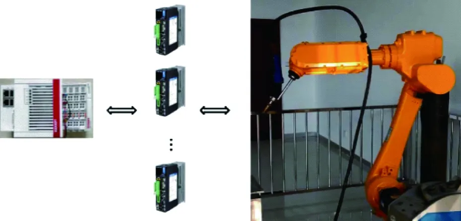
Fig.11 The control system of a six DOF robot

To verify the feasibility of the transition method, experiments are organized as follows.

3.1 Transition between two adjacent curves

A program with two move commands is tested. Each command may be a line or a circle. The first command is set to blending mode with an appropriate TP. In order to guarantee G2 continuity and minimize the amount of calculation, a cubic Bezier curve is used for transition between two lines and a quartic Bezier curve is used for transition involving one or two circles. The sample tests are shown in Figs12～14. The TP parameters are all set to 5. The transition curve with a smaller TP stays closer to the original trajectory which leads to a smaller transition error and a limited smoothness, and vice versa. The method shows good adaptability no matter where the end point of the second command is set.

3.2 Velocity and acceleration analysis

Multiple lines and circles are tested in this experiment, as shown in Fig.15. A transition curve is inserted between each pair of adjacent curves. The velocity and acceleration of the trajectory are shown in Fig.16.

Fig.12 The transition between two lines (cubic Bezier curve)

Fig.13 The transition between a line and a circle (quartic Bezier curve)

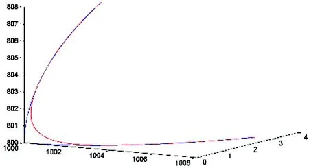
Fig.14 The transition between two circles (quartic Bezier curve)

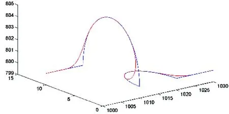
Fig.15 The transition between multiple curves

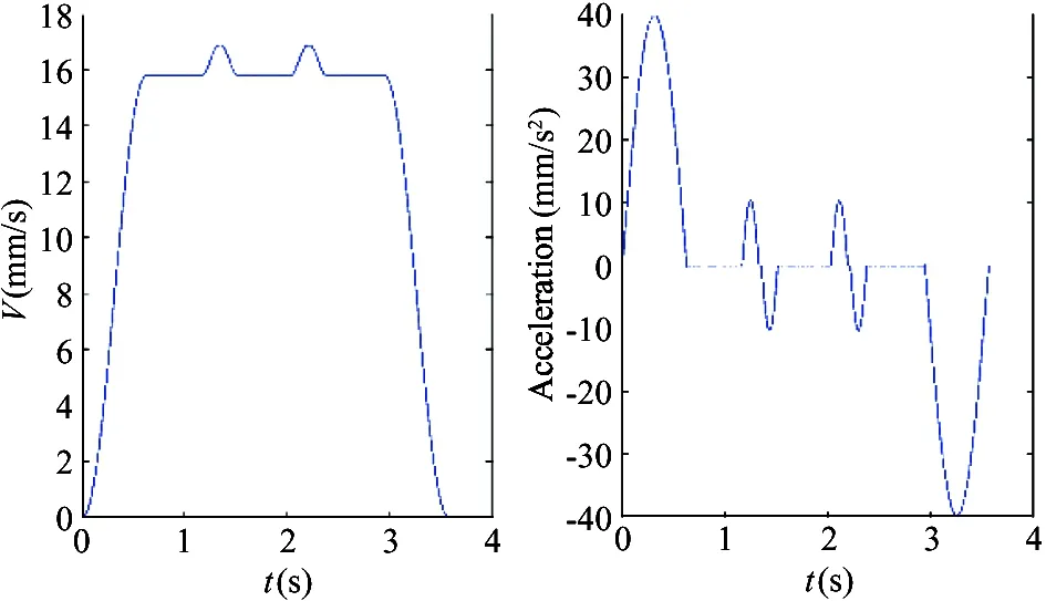
Fig.16 The velocity and acceleration of the trajectory with transition

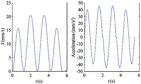
Fig.17 The velocity and acceleration of the trajectory without transition

S-curve-type acceleration profile is adopted for the velocity and acceleration planning. The maximum velocity for each curve is 50 mm/s, max acceleration is 100 mm/s2and maximum jerk is set to 200 mm/s3. The whole trajectory takes about 3.57s. The velocity and acceleration of the original trajectory without transition are shown in Fig.17. It is tested with the same velocity, acceleration and jerk constraints, and takes about 5.48s. Obviously, the velocity of the trajectory with transition is smoother and takes less time.

3.3 Velocities in the joint space

Since the trajectory of a robot is finally realized in the joint space, the position and velocity of each joint are tested. When the robot moves along the trajectory shown in Fig.15, the position of each joint can be got by inverse kinematics, and the velocity is the differential of position. Figs18～19 show the joint angle and velocity when transition mode is set to blending, and Figs20～21 show those without transition. The same result can be got that the trajectory with transition moves smoother and takes less time.

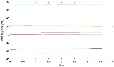
Fig.18 The joint angle corresponding to the trajectory with transition in Fig.15 (axis 1; axis 2; axis 3; axis 4; axis 5; axis 6)

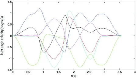
Fig.19 The joint angle velocity corresponding to the trajectory with transition in Fig.15 (axis 1; axis 2; axis 3; axis 4; axis 5; axis 6)

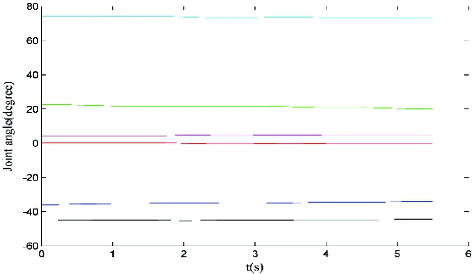
Fig.20 The joint angle corresponding to the trajectory without transition in Fig.15 (axis 1; axis 2; axis 3; axis 4; axis 5; axis 6)

4 Conclusions

It has been demonstrated that a single Bezier curve can be utilized to transit between lines and circles in three-dimensional space. In the transition between two lines, a cubic Bezier curve could satisfy the G2 continuity. In the transition between a line and a circle, if the line is coplanar with the circle, a cubic Bezier curve is able to transit smoothly. Otherwise, a quartic Bezier curve is needed. A curvature constraint is added to obtain the optimal solution in this case. In the transition between two circles, a cubic curve is hard to get the analytical solutions. So, a quartic Bezier curve is used instead. All the three situations guarantee G2 continuity with transition curve adjustable. The amount of calculation is taken into consideration in the algorithms. This method is applicable to different situations of transition between lines and circles. The velocity and acceleration of the trajectory with transition is smoother and takes less time. The same result can be got from the experiments of joint angle and joint angle velocity. Finally, future work will take more factors into consideration to get the optimal solutions for the three transition cases.

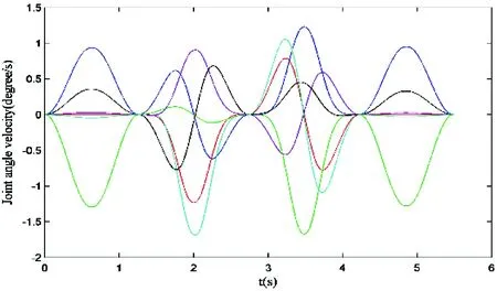
Fig.21 The joint angle velocity corresponding to the trajectory without transition in Fig.15 (axis 1; axis 2; axis 3; axis 4; axis 5; axis 6)

[ 1] PLCopen T C. Safety Software Technical Specification, Version 2.0, Part 1: Basics and Part 2-Extensions. PLCopen, Germany. 2011

[ 2] POLCopen. PLCopen Motion Control. http://www.plcopen.org/pages/tc2_motion_control: PLCopen, 2011

[ 3] Barsky B A, Derose T D. Geometric continuity of parametric curves: three equivalent characterizations.IEEEComputerGraphics&Applications, 1989, 9(6):60-69

[ 4] Sencer B, Ishizaki K, Shamoto E. A curvature optimal sharp corner smoothing algorithm for high-speed feed motion generation of NC systems along linear tool paths.InternationalJournalofAdvancedManufacturingTechnology, 2014, 76(9):1977-1992

[ 5] Bi Q, Wang Y, Zhu L, et al. A Practical continuous-curvature Bézier transition algorithm for high-speed machining of linear tool path. In: Proceedings of the 2011 International Conference on Intelligent Robotics and Applications, Aachen, Germany, 2011. 465-476

[ 6] Zhao H, Zhu L M, Ding H. A real-time look-ahead interpolation methodology with curvature-continuous B-spline transition scheme for CNC machining of short line segments.InternationalJournalofMachineTools&Manufacture, 2013, 65(2):88-98

[ 7] Hota S, Ghose D. Optimal transition trajectory for waypoint following. In: Proceedings of the 2013 IEEE International Conference on Control Applications, Hyderabad, India, 2013. 1030-1035

[ 8] Fan W, Lee C H, Chen J H. A realtime curvature-smooth interpolation scheme and motion planning for CNC machining of short line segments.InternationalJournalofMachineTools&Manufacture, 2015, 96:27-46

[ 9] Bi Q Z, Shi J, Wang Y H, et al. Analytical curvature-continuous dual-Bézier corner transition for five-axis linear tool path.InternationalJournalofMachineTools&Manufacture, 2015, 130: 96-108

[10] Ziatdinov R, Yoshida N, Kim T W. Fitting G2 multispiral transition curve joining two straight lines.Computer-AidedDesign, 2012, 44(6):591-596

[11] Habib Z, Sakai M. G2, cubic transition between two circles with shape control.JournalofComputational&AppliedMathematics, 2009, 223(1):133-144

[12] Ahmad A, Gobithasan R, Ali J M. G2 Transition curve using Quartic Bézier curve. In: Proceedings of the 2007 International Conference on Computer Graphics, Imaging and Visualization, Bangkok, Thailand, 2007. 223-228

[13] Rashid A, Habib Z. Gear tooth designing with cubic Bézier transition curve. In: Proceedings of the Graduate Colloquium on Computer Sciences, Lahore, Pakistan, 2010. 4:17

[14] Cai H H, Wang G J. A new method in highway route design: joining circular arcs by a single C-Bézier curve with shape parameter.JournalofZhejiangUniversity-ScienceA:AppliedPhysics&Engineering, 2009, 10(4):562-569

[15] Barr A H, Currin B, Gabriel S, et al. Smooth interpolation of orientations with angular velocity constraints using quaternions.AcmSiggraphComputerGraphics, 1997, 26(2):873-877

Zhang Shaolin, born in 1988. He is a Ph.D student in Institute of Automation, Chinese Academy of Sciences. He received his B.S and M.S degrees in Huazhong University of Science and Technology in 2010 and 2013 respectively. His research interests include the intelligent robotics and motion control technology.

10.3772/j.issn.1006-6748.2017.02.004

①Supported by the National Natural Science Foundation of China (No. 61573358) and Research and Development of Large Multi-function Demolition Equipment in Disaster Site(No. 2015BAK06B00).

②To whom correspondence should be addressed. E-mail: shuo.wang@ia.ac.cn

on May 17， 2016***