Wei Yang (杨炜)

College of Mechanical Engineering, Ningbo University of Technology, Ningbo 315010, China, E-mail: wyang3715@sina.com

Optimal contract wall for desired orientation of fibers and its effect on flow behavior*

Wei Yang (杨炜)

College of Mechanical Engineering, Ningbo University of Technology, Ningbo 315010, China, E-mail: wyang3715@sina.com

2017,29(3):495-503

The orientation of suspended fibers in the turbulent contraction is strongly related to the contraction ratio, which in some cases may be detrimental to the actual production. Here for a certain contraction ratio, the contraction geometry shape is optimized to obtain the desired fiber orientation. In view of the nonlinearity and the complexity of the turbulent flow equations, the parameterized shape curve, the dynamic mesh and a quasi-static assumption are used to model the contraction with the variable boundary and to search the optimal solution. Furthermore the Reynolds stress model and the fiber orientation distribution function are solved for various wall shapes. The fiber orientation alignment at the outlet is taken as the optimization objective. Finally the effect of the wall shape on the flow mechanism is discussed in detail.

Fibers orientation, wall shape, turbulent contraction, dynamic mesh, nonlinear optimization

Introduction

The fiber filling can effectively improve the stiffness and the strength of manufactured goods, whose performances depend largely on the fiber orientation distribution. The contraction is one of common internal flows, mainly used for the speedup flow, such as the pulp flow box in the paper industry and the jet nozzle of the extrusion die. It is shown that the flow behaviors inside the contraction are more complex than in the channel due to the acceleration effect, which leads to a higher alignment of the fiber orientation under the same entrance conditions. And what’s more, the fiber orientation might very likely to follow the flow direction for a large contraction ratio C because the strong streamwise strain rate, rather than the stochastic turbulence effect, would play a major rolein the vector field at this moment. As the fiber orientation alignment may affect the overall properties of the industrial products significantly, it is very important to investigate how to control the fiber orientation under a given large contraction ratio.

The dynamics of the fiber suspension and the orientation behavior of the fibers suspended in the planar contraction were much studied. Batchelor and Proudman[1]and Ribner and Tucker[2]considered the cases when C is very large and the time scale of the flow is much smaller than that of the vortex, and suggested that the development of the turbulent kinetic energy is dependent on the local flow strain rate which is related to the geometry of the flow field. Hussain and Ramjee[3]concluded that the flow shape and the Reynolds number in the axial symmetric contraction flow have little effect on the turbulent characteristics, but the inlet condition is the most important parameter. A series of studies by Lin et al.[4-8]show that with the increase of the Reynolds number more fibers will be aligned with the flow direction in the laminar flow regime while the fiber orientation distributions become more homogeneous in the turbulent regime. For the fibers with a high aspect ratio the mean velocity distribution has a more significant effect on the fiber orientation distribution than the fluctuating velocity. Olsonet al.[9,10]calculated the fiber orientation distribution with a constant diffusion coefficient in the contraction and it is shown that the influence of the contraction ratio on the fiber orientation is more significant than the entrance velocity. Parsheh et al.[11,12]employed a model with the rotational diffusion rate depending heavily on the turbulence of the entrance and decaying exponentially with the contraction ratio. Then four contraction wall shapes, including the constant mean rate of strain, the linear rate of strain, the quadratic rate of strain and the flat walls, were considered to analyze the influence of the contraction geometry on the orientation anisotropy. It is shown that the anisotropic orientation of fibers is dependent on the contraction wall shape while both the turbulence intensity and the rotational diffusion coefficient have little to do with the contraction shape. And what’s more, the rotational Peclet number, defined as the streamwise velocity gradient divided by the rotational diffusion coefficient, is shown to be the crucial quantity to determine whether the turbulent effect on the fiber orientation is dominant or not.

Although the optimal shape is not given finally by Parsheh et al.[11], the importance of the flow morphology for the motion and orientation of fibers is shown by the fact that the contraction with flat walls has the smallest orientation anisotropy and the contraction with the constant rate of strain has the largest anisotropy at the outlet . Thus the optimization of the wall shape is the way to deal with the anisotropic distribution of fibers under a constant contraction ratio, just as did by Mäkinen and Hämäläinen[13], Nazemi and Farahi[14]and Farhadinia[15]. Mäkenin and Hämäläinen[13]discretized the contaction shape with the Bezier function and solved the diffusion–convection equation with the streamline upwind Petrov-Galerkin (SUPG) finite element method. Nazemi and Farahi[14]and Farhadinia[15]turned the shape optimization problem into the coefficient optimization of the state equation, which is related to the average flow velocity gradient and the fiber orientation angle. By using an embedding method, the optimal measure representing the optimal shape is approximated by the solution of a linear programming problem. But the assumption of the quasi one dimensional potential flow was made and the effect of turbulence was neglected in their optimization solutions.

For the nonlinear and multi-variable coupling trait of the turbulence control equation, the latest optimization methods for the wall shape are mainly divided into two major categories. One is the reverse design method with the design variables obtained to meet a given objective function value by solving the control equations or by a progressive approach. But this method brings about many technical problems in practical applications: (1) It is difficult to obtain the relationship directly between the variables and the objective function, because a variable is often coupled with other variables in a group of turbulence dynamics equations. (2) The solution of the turbulent dynamics equation would be very sensitive to the mutative flow state or the boundary. Therefore, the inverse design method faces problems of sensitivity and uncertainty of the solution. (3) The method requires some relevant experience or parameters to initialize, which would make the solutions fall into a small range and make the whole optimization system lack of robustness.

The other is the optimal design method. The optimal solution with respect to the objective function can be obtained by combining the direct solution with the optimization searching of the solution space with a good performance in the practice[16,17]. But this method often uses a deputy model or an approximate calculation model, associated with the number of parameters, the sample size, the variable range and the approximate precision, and the method still needs to be adjusted and tested repeatedly for the optimization accuracy and reliability.

In order to achieve the accuracy of the dynamics solution, the deputy model is not used here. The dynamic mesh technology is adopted to model the variable flow boundary and to obtain directly the solution of the fiber orientation distribution in the turbulence. Then a parametric curve equation of the wall shape as Fig.1 is constructed at first. Based on the dynamic mesh model and the quasi-static assumption, the optimal parameters of the wall geometry can be obtained for the desired fiber orientation distribution. The effects of the wall shape parameters of the contraction, such as the inlet tangential angle a, the outlet tangential angle b and the ratioLR of the length L to the height0h, on the flow behavior are studied in detail.

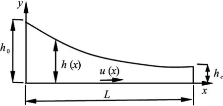
Fig.1 The 2-D model of plannar contraction

1. Parametric optimal model

1.1 Parametric equation of wall shape

Based on the bicubic parametric curves, the quintic curve, and the Vyshinsky curve for the contraction section of the wind tunnel, the parametric cubic curve for the wall shape function is constructed as follows

where0h andeh are the heights of the inlet and the outlet, respectively, and L is the length of the contraction, as shown in Fig.1. The parameters a, b, c and d can be determined to meet the boundary conditions and its first order derivative conditions:

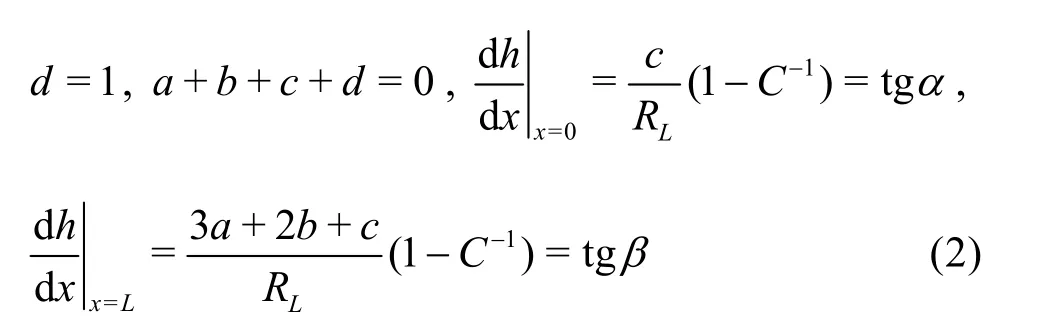
where C is the contraction ratio of h0to heand RL=L/h0.

The coefficients a, b and c in the Eq.(2) depend on the parameters a, b andLR of the boundary conditions, so various shapes of the wall surface can be obtained by adjusting these three parameters.

1.2 Optimization model

The probability distribution f(x,j) of the fiber orientation at the center streamline of the contraction can be calculated as[18].

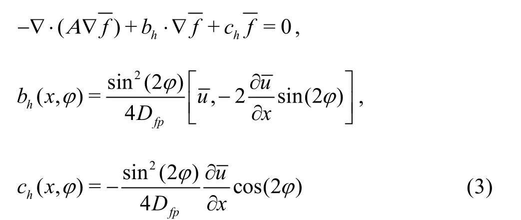
where A is the positive definite matrix, =[0,1]A ,hb andhc are the coefficient matrices, j is the orientation angle of the fibers, andfpD is the orientation diffusion coefficient of the fibers.

Optimization objective function is as follows:

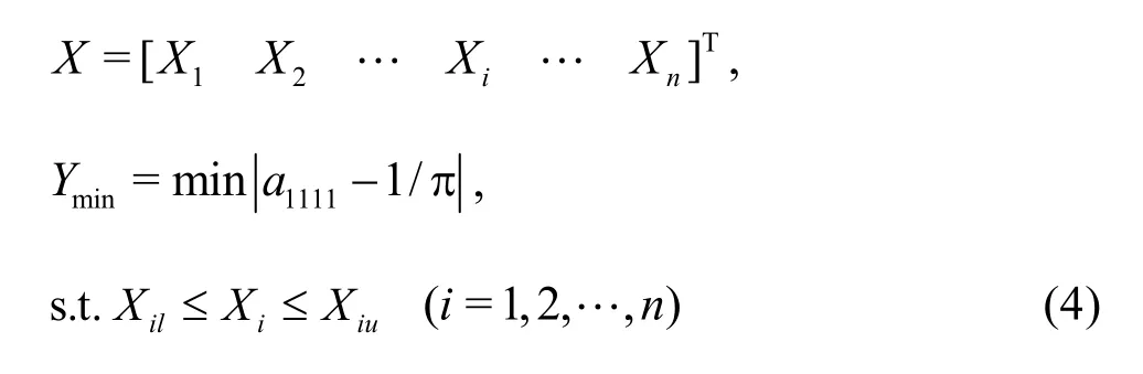
whereiX is the parameter variable to be optimized, such as a, b and c in Eq.(2).1111a is the anisotropic index of the fiber orientation, defined as1111=aHereip is the thi component of p =[cosj, sin j]T.

1.3 Dynamic mesh model

The body-fitted grid method, the arbitrary Lagrange-Euler method and the immersed boundary method are the common methods for the flow with the variable boundary, and a large number of flow problems are solved by these methods[19-21], such as those of the complex surface fluid, the dynamic boundary, the free or elastic surface and the flow field interface interaction. It is noted that these three methods are generally applied to the simulations of the low Reynolds number movement. For the turbulence problems with a high Reynolds number, these methods do not perform well due to the complexity of the coordinate transformation or the force source term for the turbulence model. In this paper the dynamic mesh technique is adopted to solve the RMS equation for the small deformation boundary.

1.4 Spring-based smoothing method

The spring-based smoothing method is utilized to realize the deformation of the dynamic mesh. At first the edges between any two mesh nodes are idealized as a network of interconnected springs, as shown in Fig.2. Hereijk is the spring constant between node i and its neighbor j,

Fig.2 Spring-based smoothing algorithm model

Based on the Hookʼs Law and the force-balance principle, an iterative equation is applied as Eq.(5). The positions of the mesh nodes are updated as Eq.(6) until convergence.

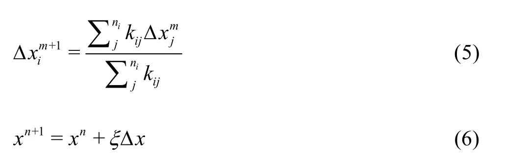
where x is the relaxation factor of the mesh nodes.x =0 means that the nodes in the mesh are not movable.

1.5 Remeshing method

When the node displacement is larger than thelocal cell sizes, the cell quality might deteriorate and the mesh distortion will even generate negative cell volumes, which would cause convergence problems. The local remeshing method is required to circumvent the problem.

There are two criteria for the local remeshing. One is the cell distortion rate, the other is the cell size. Once the cell distortion rate is greater than a specified maximum value or the cell size exceeds the range between the specified minimum length scale and the maximum length scale these bad cells would be marked and be locally updated with the new cells.

1.6 Quasi-static assumption

The isotropic orientation distribution of the fibers is expected at the outlet of the contraction by optimizing the wall shape, which is essentially to obtain the optimal steady state solution of the fiber orientation distribution under the boundary conditions of different geometric shapes. In fact the boundary is not in motion during the search for the solution, so it is necessary to introduce the quasi-static hypothesis. According to the dynamic mesh and the conservation equations, the parameter m is used to control the boundary displacement to eliminate the influence of the non steady state term for the cell motion on the solution of the conservation equation. When the flow boundary changes from one curve to the other curve, it should undergo the process of a slow variation m times to reach the steady state, to meet the quasi-static condition.

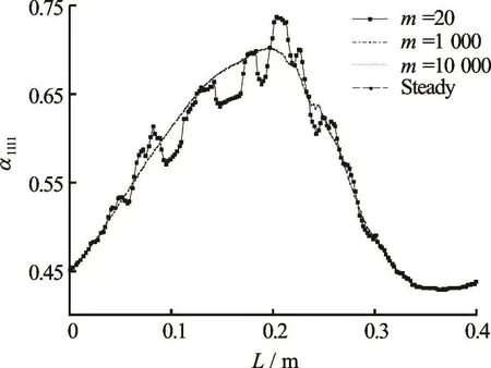
Fig.31111a under different parameters m

Figure 3 shows the solution of the fiber orientation distribution1111a along the center streamline with the steady state model and the dynamic mesh model of m =20, m =1000, m =10000. It can be seen obviously that when =20m ,1111a oscillates up and down around its steady-state solution, especially in the front pathway with a great shape change. And when m takes a larger value, such as =m 1 000 and =m 10 000, the solution of1111a is basically consistent with the steady-state solution. That is to say, the effect of the boundary motion on the solution can be eliminated. In view of the iteration efficiency, we take =m 1 000.

2. Optimal solution and discussion

2.1 Impact of wall shape parameters on1111a

In order to understand the impact of the parameters of the wall shape on the fiber orientation distribution a1111in the contract turbulence, three parameters take three levels, as shown in Table 1. According to the method of the orth4ogonal experiment design, an orthogonal table L9(3) with three factors and three levels is constructed as in Table 2. The fiber orientation distribution a1111is calculated using Eq.(3) for the nine cases, some results are shown in Fig.4.

Table 1 The levels of parameters for wall shape

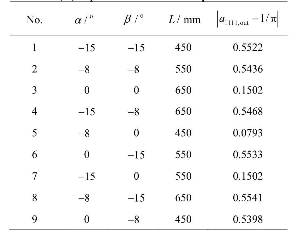
Table 2 L9(34) of parameters for wall shape

It can be seen clearly from Fig.4 that the profile of a1111changes correspondingly with the shape of the wall. The greater the b is, the larger the a1111will be. As known in Table 2,a1111,out- 1/p reaches the minimum value when a= -8o, b= 0oand RL=5.02. The influence order of the parameters on the optimal object can be obtained as in Table 3 by using the range analysis method.

Fig.4 The distribution of1111a for different walls in L9(34)

As shown in Table 3, the tangential angle b at the outlet is the leading factor to affect the optimal object a1111,out- 1/p, the next is the field length L and the tangential angle a at the inlet. The fiber orientation distribution at the outlet is the best when b= 0o. Here b is made identically equal to zero to simplify the number of parameters. As a result, the number of the optimal variables changes from three to two, i.e., the field length L and the inlet tangential angle a. Thus the variable range can be adjusted to 350mm£L£ 650mm , a would be in the appropriate range of [-4 0o,0o] according to the channel length L.

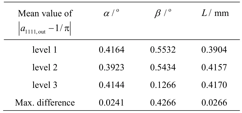
Table 3 Analysis results ofa1 111,out - 1/p

2.2 Optimal shape parameters

According to the scope of the above parameters, various wall shapes are generated by using the dynamic mesh method and the fiber orientation distribution a1111is calculated by Eq.(3) using the inlet data in Table 4, which is the same as in Parsheh’s case. The distribution map of a1111is listed only in the field of L =350mm and -4 0o＜a＜0oas follows.

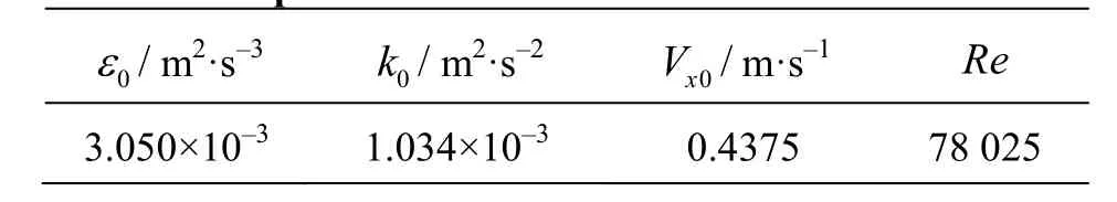
Table 4 Inlet parameters of the contract flow

It is known that from the trend of1111a in Fig.5 the largest contraction occurs at the inlet at first and then moves forward gradually to a place near the outlet when a changes from the maximum negative angle to zero and the field length L remains constant. Accordingly, the maximum alignment index1111a of the fiber orientation distribution also varies with the contraction trend of the wall shape. Although the flow length L and the tangent angle a at the inlet take different values in each numerical case, the maximum value of a1111no longer occurs at the outlet but in the front of the outlet without exception due to the tangent angle b= 0oat the outlet. And what’s more, a1111values are all close to the average probability distribution, i.e., 1/p, at the outlet which indicates that1111a is effectively controlled in the contraction. Of course in addition to the main effect of b on the fiber orientation, the parameters L and a still have a subtle influence on the maximum value a1111,maxof the fiber orientation distribution and the average value a1111,outat the outlet.

The values of a1111,maxand a1111,out- 1/p are shown in Fig.6 and Fig.7 for the different cases. a1111,maxcan take the minimum when the parameters L =550mmand a= -1 0o.a1111,out- 1/p can take the minimum when the parameters L =350mm anda =0o. Thus it can be seen that when the wall shape is close to the linear contraction line, the fiber orientation a1111,maxwould be relatively smaller, that is to say, the wall shape near the linear contraction can reduce the fiber alignment in the contract flow. From Fig.7a1111,out- 1/p all can reach the lowest point at the outlet in the cases of a= 0o, which suggests that the fi ber orienta tio n cou ld exh ibit a better isotropy . In ordertoobtainagoodresultof a1111,out- 1/p,thelength of the flow does not seem to need too long, and a slightly shorter length seems more appropriate. If only for the purpose of a1111,out- 1/pmin, the wall curve with the parameters of L =350mm , a=0oand b= 0ois optimal.

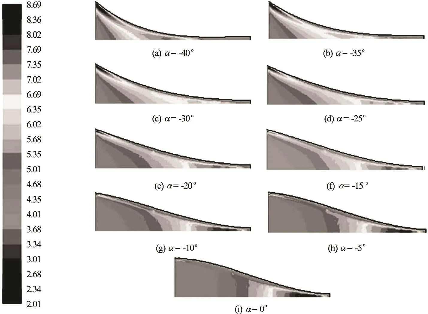
Fig.5 The distribution of a1 111for L =350mm and different a

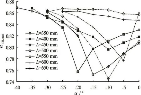
Fig.6 The variation of a1 111,maxfor different a and L

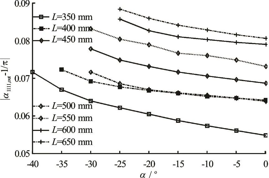
Fig.7 The variation of a1 111,out - 1/p for different a and L

Fig.8 Turbulent intensity along the center streamline for different a and L=550mm

2.3 Flow mechanisms and shape parameters

2.3.1 Impact of a on flow behavior

It is easy to see from Eq.(3) that the fiber orientation distribution is mainly controlled by the evolution of the velocity gradient and the flow structure in the flow field. The variation of the boundary shapecan change the velocity gradient directly, and a large velocity gradient is one of the main factors to generate a large scale turbulence vortex. The curve of the turbulent structure along the center streamline is obtained by numerical simulations, as shown in Fig.8, when the channel length L =550mm and the inlet tangential angle a takes various values from a= -3 0otoa= 0o.

The turbulent intensity is the ratio of the mean square root of the turbulent fluctuation velocity to the mean velocity of the flow field. The turbulence strength and the diffusion coefficient of the turbulent transport is generally related to this index. Usually the turbulence in the range of 5%-20% is called the higher turbulence, and that in the range of 1%-5% is called the moderate turbulence; that in the range less than 1% is called the low turbulence. The natural transition, as one of the most common form of the transition, occurs in the case of the low turbulence.

From Fig.8, the turbulence intensity (T I) in general decreases at first and then increases along the center streamline. When the inlet tangential angle changes from a= -3 0oto a=0othe inflection point of different curves is more and more close to the outlet. When a= -3 0othe wall shape is transformed from the necking mouth to a tiny flaring mouth at the position of x=350mm-400mm , the turbulence intensity begins to oscillate and increase rapidly. When a approaches 0o, the curve changes gradually from oscillation to a stable state. The simulation results show that too large turbulence intensity is not appropriate for the fiber orientation distribution because it may produce a large lateral velocity and affect the flow quality.

Fig.9 Turbulent vorticity along the center streamline for different a and L=550mm

The turbulent vorticity ( )Vot is defined as the curl of the fluid velocity vector to describe usually the strength and the direction of the turbulent eddies. It is one of the most important physical quantity of the vortex motion. Figure 9 shows that the change of the vorticity with a is similar to the turbulence intensity, except that the vorticity under a linear wall is close to zero along the center streamline. It can be inferred that the tensile effect under the linear contract wall is stronger than the others, which make the vortex stretch, the vorticity be weakened and the fiber more easily align along the streamline. As a result, the phenomenon of the weak vorticity is common in the flow with a linear contract wall instead of the flow with a wall shape of large curvature variations. And due to the fact thatb=0oat the outlet, the curvature variation of the wall shape is small and the vorticity remains at the same energy level or lower on the whole.

2.3.2 Impact of L on flow behavior

Consider the inlet tangential angle a= 0oand the channel length L=350mm-650mm in the numerical simulation. The turbulence changes with the contraction ratio C along the center streamline as shown in Fig.10. Figure 10 shows that the shorter the channel length L is, the more quickly the turbulence intensity of the flow increases with the contraction ratio C at the same inlet tangential angle a, which maybe explains why the fiber orientation is inclined to the state of isotropy in a short contraction.

Fig.10 Turbulent intensity changes with C along the center streamline

Fig.11 Turbulent vorticity changes with C along the center streamline

The maximum amplitude of the turbulent vorticity and its peak position vary with the channel length L, as shown in Fig.11. The maximum peak in the flow field of L =400mm occurs at C =9, its amplitude is about 8 s‒1, then, the maximum peak of L= 500 mm occurs almost at C =7.5 and its amplitude is about 6.5 s‒1. The maximum peaks of L =450mm, L =600mm and L =650mm occur near the place C =11, its amplitude is about 5 s‒1. The maximum peak of L =350mmoccurs near the place C =8.5, its amplitude is also about 5 s‒1. The maximum peak of L =550mm occurs near the place C =11, its amplitude is also about 4.5 s‒1. Finally the maximum peak in the linear contraction of L =550mm occurs at the outlet, its amplitude is only about 2 s‒1. Although from Fig.11 it is not sure about the certain relationship between the channel length L and the peak magnitude of the vorticity, it can be concluded that the maximum amplitude of the turbulence vorticity very likely occurs slightly away from the outlet in order to reduce the orientation alignment of the fibers.

2.3.3 Impact of a and L on Peclet number

Parsheh’s study[11]shows that the rotating Peclet number ( )Pe is effective to assess the impact of the turbulence on the fiber anisotropic orientation. It can be defined as the ratio of the local velocity gradient to the rotational diffusion coefficient. The influence of the turbulence on the fiber orientation can be ignored when Pe> 10 and the fiber orientation tends to be isotropic when C＜4 and Pe is very small. Here the Peclet number is used to explain effectively the effect of the wall shape on the flow mechanisms and the fiber orientation behavior.

Fig.12 The variation of Pe along the cental streamline for different a and L=550mm

Figure 12 shows that the Peclet number evolves along the center streamline for different inlet tangential angle a for a given channel length L =550mm . When a changes from a= -3 0oto a= 0o, the wall shape turns from a concave curve to a first-convexthen-concave curve, which directly varies the velocity gradient of the flow. In the first half of the contract field, the Peclet number is large when a = -3 0oand it is small when a=0owhile the situation is opposite in the second half field. Finally the Peclet numbers all remain at a low level to decrease the anisotropic orientation of the fibers significantly due to the fact thatb= 0oat the outlet except for the linear contraction. The fluctuations of the Peclet number curve just reflect the effect of the wall curvature on the velocity gradient in the flow field, so it can be inhibited to a certain extent by controlling the curvature of the wall geometry.

The Peclet number varies similarly with the contraction ratio C, but much less than the linear wall in Fig.13, where the inlet tangential angle a retains zero degree and the channel length L takes different values from 350 mm to 550 mm. The evolution of the Peclet number with the contraction ratio reflects more intuitively that the velocity gradient in the flow has the trend of first increasing and then decreasing with C. As a result, the anisotropic orientation distribution of the fibers in all the parametric contractions is smaller than in the linear contraction.

Fig.13 The variation of Pe with C along the cental streamline for different L and a=0o

3. Conclusions

The contraction ratio C is an important factor to determine the orientation distribution of suspending fibers, especially in case of a large speedup needed by the actual manufacturing. Though at present there are many methods to optimize the anisotropic orientation of the fibers, an effective method is still not easy to find to obtain a desired boundary shape based on the flow mechanism and the dynamics precision. Therefore a dynamic mesh model is established for the turbulent contraction using an adaptive grid algorithm and the quasi static hypothesis. Then the dynamics model of the turbulent flow with a variable boundary can be used by optimization objectives and the optimalparameters of the wall shape can be searched and obtained. Finally, the influence of the wall shape parameters including the inlet tangential angle, the channel length and the outlet tangential angle on the flow behavior and the fiber orientation distribution in the turbulence is analyzed and discussed. Several meaningful conclusions are drawn as follows:

(1) The essence of an optimal wall shape is the optimization of the distribution of the local velocity and velocity gradient in the flow field, to affect the diffusion and orientation behavior of suspending fibers and then consequently to obtain the desired fiber orientation distribution. The inlet tangential angle a, the channel length L and the outlet tangential angle bare three parameters to control the contract shape of the wall. When b= 0oand the wall shape is very close to the linear contraction, a1111,maxachieves the minimum but a1111,out-1/p is not optimal. Whenb =0o, a = 0oand the channel length L is slightly short,a1111,out-1/p assumes the minimum value and is optimal. How to explain these results? The outlet is similar to a short straight channel at b= 0oand the tensile effect of the straight channel flow is much smaller than that of the contraction so that the fibers are no longer strongly under the stretching action of the flow field but take various orientations under the turbulent effect. The inlet tangential angle a and the channel length L can control the position of the maximum velocity gradient in the flow field, so they can adjust the value and the occurrence location of a1111,max.

(2) The velocity gradient increases almost linearly with the contraction ratio and the tensile effect of the mean flow is much stronger than the random effect of the turbulence in the linear contract flow field, which make the fibers easy to align with the streamline consequently. In contrast, the variation of the velocity gradient with the boundary curvature is not monotonic in the flow field with the parametric surface. The non monotonic variation of the curvature would have the random effects of the turbulence enhanced to a certain extent and the fibers would have more chances of random orientations. Finally the orientation alignment of the fibers at the outlet can be improved in the contraction.

[1] Batchelor G. K., Proudman I. The effect of rapid distortion of a fluid in turbulent motion [J]. Quarterly Journal of Mechanics and Applied Mathematics, 1954, 7(1): 83-103.

[2] Ribner H., Tucker M. Spectrum of turbulence in a contracting stream [R]. Technical Report Archive and Image Library, 1953, 99-115.

[3] Hussain A. K., Ramjee V. Effects of the axisymmetric contraction shape on incompressible turbulent flow [J]. Journal of Fluids Engineering, 1976, 98(1):58-68.

[4] Lin J. Z., Zhang L. X. On the structural features of fiber suspensions in converging channel flow [J]. Journal of Zhejiang University-Science A, 2003, 4(4): 400-406.

[5] Lin J., Shi X., You Z. Effects of the aspect ratio on the sedimentation of a fiber in Newtonian fluids [J]. Journal of Aerosol Science, 2003, 34(7): 909-921.

[6] Lin J., Shi X., Yu Z. The motion of fibers in an evolving mixing layer [J]. International Journal of Multiphase Flow, 2003, 29(8): 1355-1372.

[7] Lin J., Zhang W., Yu Z. Numerical research on the orientation distribution of fibers immersed in laminar and turbulent pipe flows [J]. Journal of Aerosol Science, 2004, 35(1): 63-82.

[8] Lin J., Liang X., Zhang S. Fibre orientation distribution in turbulent fibre suspensions flowing through an axisymmetric contraction [J]. Canadian Journal of Chemical Engineering, 2011, 89(12): 1416-1425.

[9] Olson J. A. The motion of fibre in turbulent flow, stochastic simulation of isotropic homogeneous turbulence [J]. International Journal of Multiphase Flow, 2001, 27(12): 2083-2103.

[10] Olson J. A. Frigaard I., Chan C. et al. Modeling a turbulent fibre suspension flowing in a planar contraction: The onedimensional headbox [J]. International Journal of Multiphase Flow, 2004, 30(1): 51-66.

[11] Parsheh M., Matthew L. B., Cyrusk A. On the orientation of stiff fibres suspended in turbulent flow in a planar contraction [J]. Journal of Fluid Mechanics, 2005, 545: 245-269.

[12] Parsheh M., Brown M. L., Aidun C. K. Variation of fiber orientation in turbulent flow inside a planar contraction with different shapes [J]. International Journal of Multiphase Flow, 2006, 32(12): 1354-1369.

[13] Mäkinen R. A. E., Hämäläinen J. Optimal control of a turbulent fibre suspension flowing in a planar contraction [J]. Communications in Numerical Methods in Engineering, 2010, 22: 567-575.

[14] Nazemi A. R., Farahi M. H. Control the fibre orientation distribution at the outlet of contraction [J]. Acta Applicandae Mathematicae, 2009, 106(2): 279-292.

[15] Farhadinia B. Planar contraction design with specified fibre orientation distribution at the outlet [J]. Structural and Multidisciplinary Optimization, 2012, 46(4): 503-511.

[16] Ye S., Xiong J. Geometric optimization design system incorporating hybrid GRECO-WM scheme and genetic algorithm [J]. Chinese Journal of Aeronautics, 2009, 22(6): 599-606.

[17] Zhang Z., Ding Y., LIU Y. Shape optimization design method for the conceptual design of reentry vehicles [J]. Acta Aeronautica Et Astronautica Sinica, 2011, 32(11): 1971-1979.

[18] Yang W. A new method for fiber orientation distribution in a planar contracting turbulent flow [J]. Thermal Science, 2012, 16(5): 1367-1371.

[19] Yang J. Sharp interface direct forcing immersed boundary methods: A summary of some algorithms and applications [J]. Journal of Hydrodynamics, 2016, 28(5): 713-730.

[20] Feng Z. R., Wang L. X., Cui J. H. Research on the generation of two-dimensional fitted-body grid by adjacent boundary nodes sliding method [J]. Advanced Materials Research, 2013, 651: 835-840.

[21] Xu W., Chen G., Deng Z. et al. The dynamical design of a steel frame based on the arbitrary Lagrange-Euler method [J]. Structures Under Shock and Impact XIII, 2014, 141: 51-57.

10.1016/S1001-6058(16)60761-8

February 27, 2016, Revised May 18, 2016)

* Project supported by the National Natural Science Foundation of China (Grant No. 11302110), the Public Project of Science and Technology Department of Zhejiang Province (Grant No. 2015C31152), the Natural Science Foundation of Ningbo (Grant No. 2014A610086) and “Wang Weiming”Entrepreneurship Supporting Fund.

Biography:Wei Yang (1975-), Female, Ph. D.,

Associate Professor