Jie-min Zhan (詹杰民), Wen-qing Hu (胡文清), Wen-hao Cai (蔡文豪), Ye- jun Gong (龚也君), Chi-wai Li (李志伟)

1.Department of Applied Mechanics and Engineering, School of Engineering, Sun Yat-Sen University, Guangzhou 510275, China, E-mail: cejmzhan@vip.163.com

2.Department of Civil and Environmental Engineering, Hong Kong Polytechnic University, Hong Kong, China

(Received November 29, 2016, Revised December 15, 2016)

Numerical simulation of flow through circular array of cylinders using porous media approach with non-constant local inertial resistance coefficient＊

Jie-min Zhan (詹杰民)1, Wen-qing Hu (胡文清)1, Wen-hao Cai (蔡文豪)1, Ye- jun Gong (龚也君)1, Chi-wai Li (李志伟)2

1.Department of Applied Mechanics and Engineering, School of Engineering, Sun Yat-Sen University, Guangzhou 510275, China, E-mail: cejmzhan@vip.163.com

2.Department of Civil and Environmental Engineering, Hong Kong Polytechnic University, Hong Kong, China

(Received November 29, 2016, Revised December 15, 2016)

Aquatic vegetation zone is now receiving an increasing attention as an effective way to protect the shorelines and riverbeds. To simulate the flow through the vegetation zone, the vegetation elements are often simplified as equidistant rigid cylinders, and in the whole zone, the porous media approach can be applied. In this study, a non-constant inertial resistance coefficient is introduced to model the unevenly distribution of the drag forces on the cylinders, and an improved porous media approach is applied to one circular array of cylinders positioned in a 2-D flume. The calculated velocity profile is consistent with the experimental data.

Vegetation zone, cylinder array, porous media, inertial resistance coefficient

The aquatic vegetation is widely researched due to the significant influence on ecosystem and hydraulics. On the aspect of laboratory experiments, a series of classic experiments were conducted by Ghisalberti and Nepf[1]and Nezu and Onitsuka[2]. In their studies, the vegetation is simulated by rigid bodies, and the whole vegetation zone is regarded as an array of solid cylinders. The tracking dye is used to track the flow trajectory, showing the complex flow pattern, turbulence and diffusion in the flows through the vegetation.

For the numerical simulation, two main methods[3]are widely employed to simulate the flow through the vegetation. The first method, which resolves the flow around each vegetation unit, is called the multi-body model[4]. Each vegetation unit is generallysimplified as a cylinder and each one of them is taken into consideration in the model. The second method, the porous model[5], treats the entire vegetation zone as a porous zone and the impact of the vegetation on the flow is governed by the relevant parameters of the porous zone. Compared with the porous model, the multi-body model considers the influence of each single vegetation unit, therefore, is more accurate and time consuming. Relatively speaking, as the porous model regards the vegetation as one porous zone, the computational efficiency is better, therefore, it is more widely used in the real engineering applications.

For the flow of incompressible, homogeneous and viscous fluid, the governing Navier-Stokes equations can be written as

wherevis the velocity vector,ρis the fluid density,pis the pressure,νis the kinematic viscosity,Fbrepresents the force acting on the unit mass and it is generally related to the gravitational accelerationg.

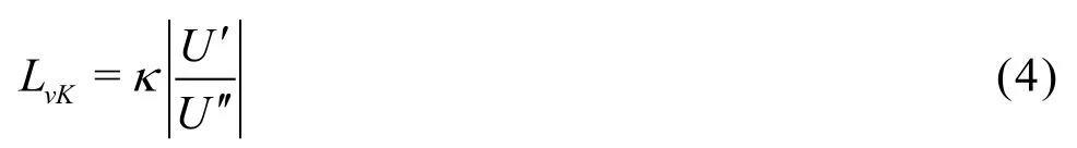
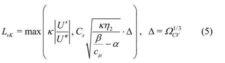
A hybrid RANS/LES turbulence model, the scale adaptive simulation (SAS) model, is employed. The SAS model is based on the SST model, which behaves very much like thek-ωmodel away from the wall and serves to control the turbulence level in the near wall region. But the length scale produced by the SST model is too large. To avoid this shortcoming, in the SAS model, the von Karman length scale is introduced into the turbulence scale equation, such that the turbulence length-scale can be resolved correctly. The transport equations for the SAS model are defined as[8]

The additional source termQSASis defined as

The porous media are modeled by adding one source term to the momentum equations. The source term is composed of two parts: a viscous loss term and an inertial loss term. For homogeneous porous media, the source term is defined as

whereαis the permeability andC2is the inertial resistance factor. This momentum sink contributes to the pressure gradient in the porous cell.

In the convectional porous model, the inertial resistance factor is assumed to be constant. However, it is in conflict with the real situation, especially, when the size of the porous region is large. In this study, two assumptions are made in the porous region of the cylinder array: the local inertial resistance is proportional to the local pressure drop, the pressure head loss along the flow direction can be neglected. With these assumptions, the local inertial resistance can be redefined as

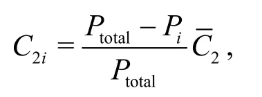
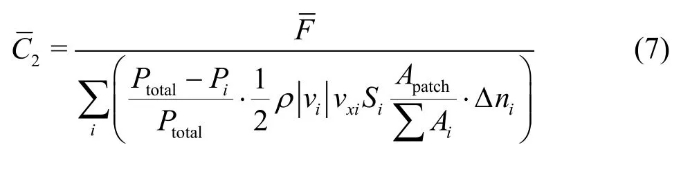
whereC2iis the inertial resistance coefficient in celli, and2is the averaged coefficient value in the area of the circular patches.Ptotalis the total pressure on the inlet boundary,Piis the local cell static pressure,is the time-averaged drag force of the circular patches,is the velocity magnitude,vxiis the velocity in the flow direction,Siis the cross sectional area of the local cell normal to the flow direction,Apatchis the area of the circular patches,∑Aiis the summation of the areas of the local cells, and Δniis the thickness of the local cell.Ptotalis a constant when the inlet velocity remains the same.

In order to validate the feasibility and the rationality of the improved porous method with the adoption of the non-constant local inertial resistance coefficient, the calculated velocity field is compared to the measurements of the experiments conducted by Zong et al.[9]. The computational domain is shown in Fig.1, where the circular vegetation zone with diameterD= 0.22 m is centered atx=0. The diameter of each circular dot (vegetation unit) isd=0.006 m. The flume’s width is 1.2 m, and the water depth is 0.133 m. Additionally, two monitoring lines (marked in red in Fig.1) are set at the appropriate positions to obtain the relative velocity profiles measured in the experiments. The time-averaged horizontal velocityuis measured at liney=0, while the time-averaged vertical velocityis measured at liney=D/2, respectively. The dimensionless constantΦ=N(d/D)2(whereNrepresents the number of circular patches) is defined as the ratio of the sum of all circular patch areas to the total vegetation region area, representing the plant density of the vegetation. In the porous model, the value ofΦrepresents the porosity, andΦ=0.03both for the multi-body and the porous models in this study.

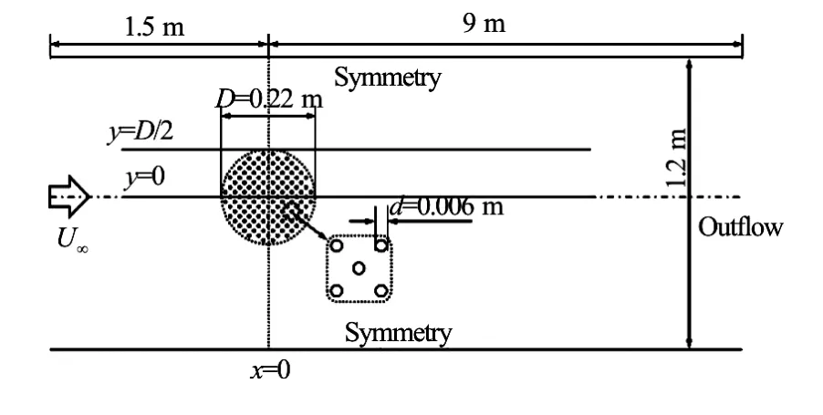
Fig.1 The schematic diagram of computational model

Fig.2 (Color online) Contour maps of the local inertial resistance coefficients

Figure 2 is the contour maps of the local inertial resistance coefficients. It is calculated based on the SAS multi-body model. As is described above, the porous model has a smaller size, that requires an interpolation of the C2 distribution inside the porous zone.

Figure 3 shows the time-averaged horizontal velocity profile along the liney=0. Similarly, Fig.4 shows the time-averaged vertical velocity profile along the liney=D/2.U∞is the inlet velocity,Dis the diameter of the circular patches. Both results of the multi-body model and the porous model fit well with the experimental data outside the circular region of the cylinder array. The multi-body model performs better in the prediction of the vertical velocity than the porous model away from the cylinders. Moreover, the multi-body model predicts the fluctuation of the flow velocity inside the region of the cylinder array, caused by impacting effect of the flow through the dense array of cylinders. Note that the distribution of thecylinders is unknown in the experiment, so the measured velocity in the region of the cylinder array is not shown in Figs.3, 4.

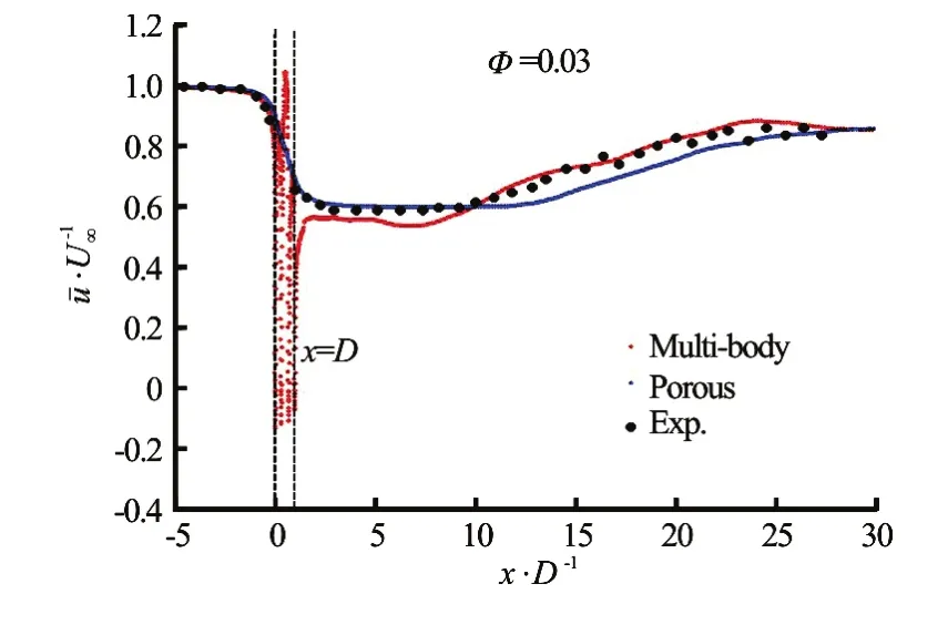
Fig.3 (Color online) Time-averaged horizontal velocity profiles alongy=0

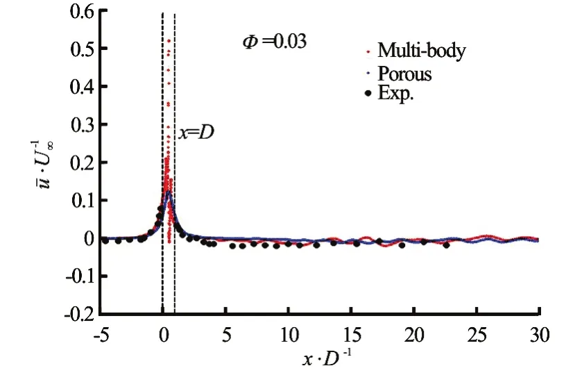
Fig.4 (Color online) Time-averaged vertical velocity profiles alongy=D/2

The vorticity fields simulated by the multi-body and porous models are shown in Figs.5, 6, where Fig.6 shows the details of the vorticity field around the cylinder array. As expected, the porous model can not capture the small scale vortices in the near-field, but still gives some details of the disturbance inside the porous zone, as shown in Fig.6. However, in the farfield, the porous model gives a similar vorticity field as the multi-body model.

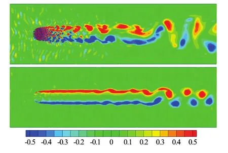
Fig.5 (Color online) Vorticity fields of multi-body (a) and porous (b) models

Fig.6 (Color online) Contours of transient vorticity magnitude near porous zone

Compared to the multi-body method, the improved porous model can give a proper result over the flow field while the simulation cost is much less than the multi-body model, such that it is suitable for the large-scale engineering applications.

[1] Ghisalberti M., Nepf H. M. Mixing layers and coherent structures in vegetated aquatic flows [J].Journal of Geophysical Research: Oceans, 2002, 107(2): 1-11.

[2] Nezu I., Onitsuka K. Turbulent structures in partly vegetated open-channel flows with LDA and PIV measurements [J].Journal of Hydraulic Research, 2001, 39(6): 629-642.

[3] Yu L. H., Zhan J. M., Li Y. S. Numerical investigation of drag force on flow through circular array of cylinders [J].Journal of Hydrodynamics, 2013, 25(3): 330-338.

[4] Zhang H., YANG J. M., XIAO L. F. et al. Large-eddy simulation of the flow past both finite and infinite circular cylinders atRe=3900[J].Journal of Hydrodynamics, 2015, 27(2): 195-203.

[5] Su X., Li C. W. Large eddy simulation of free surface turbulent flow in partly vegetated open channels [J].International Journal for Numerical Methods in Fluids, 2002, 39(10): 919-937.

[6] Yu L. H., Zhan J. M., Li Y. S. Numerical simulation of flow through circular array of cylinders using multi-body and porous models [J].Coastal Engineering Journal, 2014, 56(3): 1450014.

[7] Wang Q., Li M., Xu S. Experimental study on vortex induced vibration (VIV) of a wide-D-section cylinder in a cross flow [J].Theoretical and Applied Mechanics Letters, 2015, 5(1): 39-44.

[8] Menter F. R., Egorov Y. The scale-adaptive simulation method for unsteady turbulent flow predictions. Part 1: Theory and model description [J].Flow, Turbulence and Combustion, 2010, 85(1): 113-138.

[9] Zong L., Nepf H. Vortex development behind a finite porous obstruction in a channel [J].Journal of Fluid Mechanics, 2012, 691: 368-391.

* Project supported by the Special Fund of Marine-Fishery Science-Technology Extension in Guangdong Province (Grant No. A201401B08).

Biography:Jie-min Zhan (1963-), Male, Ph. D., Professor

Ye-jun Gong, E-mail:yejungong@126.com