LI Jin-Xi， LI Yi-Yunnd WANG Bin，c

aState Key Laboratory of Numerical Modeling for Atmospheric Sciences and Geophysical Fluid Dynamics， Institute of Atmospheric Physics，Chinese Academy of Sciences， Beijing， China；bCollege of Earth Science， University of Chinese Academy of Sciences， Beijing， China；cMinistry of Education Key Laboratory for Earth System Modeling， and Center for Earth System Science， Tsinghua University， Beijing， China

Characteristics of pressure gradient force errors in a terrain-following coordinate

LI Jin-Xia，b， LI Yi-Yuanaand WANG Bina，c

aState Key Laboratory of Numerical Modeling for Atmospheric Sciences and Geophysical Fluid Dynamics， Institute of Atmospheric Physics，Chinese Academy of Sciences， Beijing， China；bCollege of Earth Science， University of Chinese Academy of Sciences， Beijing， China；cMinistry of Education Key Laboratory for Earth System Modeling， and Center for Earth System Science， Tsinghua University， Beijing， China

A terrain-following coordinate （σ-coordinate） in which the computational form of pressure gradient force （PGF） is two-term （the so-called classic method） has signifcant PGF errors near steep terrain. Using the covariant equations of the σ-coordinate to create a one-term PGF （the covariant method）can reduce the PGF errors. This study investigates the factors inducing the PGF errors of these two methods， through geometric analysis and idealized experiments. The geometric analysis frst demonstrates that the terrain slope and the vertical pressure gradient can induce the PGF errors of the classic method， and then generalize the efect of the terrain slope to the efect of the slope of each vertical layer （φ）. More importantly， a new factor， the direction of PGF （α）， is proposed by the geometric analysis， and the efects of φ and α are quantifed by tan φ·tan α. When tan φ·tan α is greater than 1/9 or smaller than -10/9， the two terms of PGF of the classic method are of the same order but opposite in sign， and then the PGF errors of the classic method are large. Finally， the efects of three factors on inducing the PGF errors of the classic method are validated by a series of idealized experiments using various terrain types and pressure felds. The experimental results also demonstrate that the PGF errors of the covariant method are afected little by the three factors.

ARTICLE HISTORY

Revised 29 January 2016

Accepted 1 February 2016

Terrain-following coordinate；pressure gradient force

errors； direction of pressure gradient； slope of each

vertical layer； nonlinear

vertical pressure gradient；

pressure gradient along

vertical layer

“地形追随坐标系中气压梯度力误差的特征分析”一文通过几何分析和理想实验，对比了地形追随坐标系两种方案（经典方案和协变方案）中气压梯度力（PGF）误差的特征。结果表明：（1）经典方案的PGF误差受“垂直气压梯度”，“气压梯度的方向（α）”，“垂直层的坡度（φ）”三者影响，垂直气压梯度越大，气压梯度与水平方向的夹角越大，垂直层坡度越大，误差越大；（2）协变方案的PGF误差不受上述三因子影响 。此外，通过定义参数TT（TT = tanφ·tanα）能定量分析经典方案的PGF误差。

1. Introduction

Since a terrain-following coordinate （σ-coordinate） （Phillips 1957） can transform the complex surface of Earth into a regular coordinate surface， the σ-coordinate becomes a common choice for atmospheric and oceanic models. However， the computational form of pressure gradient force （PGF） in a σ-coordinate is two-term （the so-called classic method）. These two terms are opposite in sign and of the same order near steep terrain， which induces signifcant numerical errors； namely， the PGF errors of the σ-coordinate （Haney 1991； Li， Wang， and Wang 2012； Lin 1997； Ly and Jiang 1999； Shchepetkin and McWilliams 2003； Smagorinsky et al. 1967）.

Many methods have been proposed to reduce the PGF errors， which can be categorized into three types. The frst type is to reduce the PGF errors based on the two-term PGF， and includes high-order schemes （Blumberg and Mellor 1987； Corby， Gilchrist， and Newson 1972； Mahrer 1984；Qian and Zhou 1994）， standard stratifcation deduction（Zeng 1979）， and so on. The second type is to overcome the PGF errors through various coordinate transformations based on the non-orthogonal σ-coordinate （Li， Wang， and Wang 2012； Qian and Zhong 1986； Smagorinsky et al. 1967；Yan and Qian 1981； Yoshio 1968）. And the third type is to design an orthogonal terrain-following coordinate to bypass the PGF errors （Li et al. 2014）. Both methods proposed by Li， Wang， and Wang （2012） and Li et al. （2014）create a one-term computational form of PGF， while Li，Wang， and Wang （2012） proposed to use the covariant scalar equations of the σ-coordinate （the covariant method）. Note that studies on the factors inducing the PGF errors are less common than eforts made to reduce the PGF errors.

For the classic method， there are two factors inducing the PGF errors； namely， the terrain slope and the nonlinear vertical pressure gradient （Yan and Qian 1981； Zeng and Ren 1995）. Recently， Klemp （2011） proposed that the PGF errors could be minimized when the vertical pressure gradient is nearly linear. The idealized experiments implemented by Li， Li， and Wang （2015） demonstrated that the PGF errors increased according to the increasing terrain slope. However， for the covariant method， few analyses of the factors inducing the PGF errors have been carried out.

In this study， we further explore the factors inducing the PGF errors of the classic and covariant method. In Section 2 we use geometric analysis to identify all the possible factors inducing the PGF errors of the classic method. In Section 3 we implement a series of idealized experiments of various terrain types and pressure felds to investigate the efects of all the factors identifed in Section 2 that induce the PGF errors of the classic and covariant method.

2. Geometric analysis of the PGF errors of theclassic method

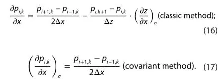
The two-term expression of PGF of the classic method is given by

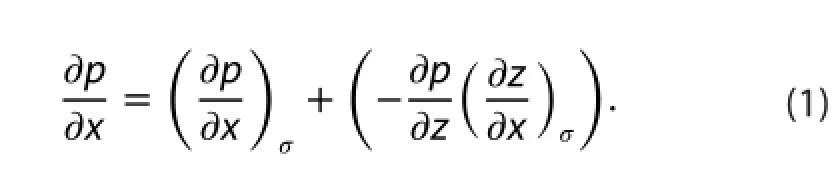
We abbreviate the frst and second term on the RHS of Equation （1） as PGF1 and PGF2， respectively. According to Equation （1）， the PGF of the classic method is relevant to three factors:

（1） The pressure gradient along each vertical layer

Since the terrain slope equals the slope of the bottom vertical layer in a model， the efect of terrain slope can be included in the efect of each vertical layer on inducing the PGF errors. The efect of the vertical pressure gradient on inducing the PGF errors has been analyzed by many researchers （e.g. Zeng and Ren 1995）. Therefore， we only investigate the efects of the pressure gradient along each vertical layer and slope of each vertical layer.

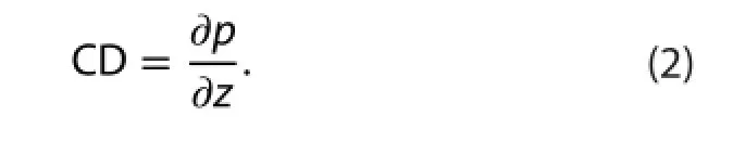
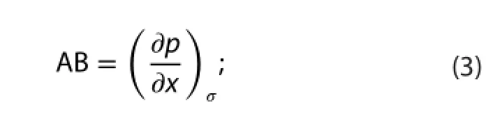
Figure 1.Schematic diagrams of PGF vectors and their components of diferent coordinates.Notes: Green curves represent a certain vertical layer； blue lines are its tangent and normal directions. S1， S2， and S3in （a） indicate the areas of diferent directions of PGF. Panels （b—d） are schematic diagrams of PGF in S1， S2， and S3， respectively. Red lines with solid arrows（AC） represents ∇p. Black- and red-arrowed lines are the components of the PGF of the σ- and z-coordinate， respectively.

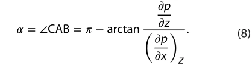
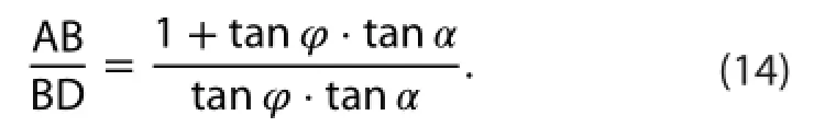
The pressure gradient along each vertical layer is AB:the direction of PGF （α） is∠CAB， and the slope of each vertical layer （φ） is given by

In addition， according to the geometric relationship in Figures 1（b）—（d）， we obtain

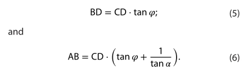
Equation （6） manifests that the pressure gradient along each vertical layer （AB） can be represented by the vertical pressure gradient （CD）， the direction of PGF （α） and the slope of each vertical layer （φ）. Therefore， the possible factors inducing the PGF errors of the classic method are as follows: （1） the direction of PGF （α）； （2） the slope of each vertical layer （φ）； （3） the vertical pressure gradient （CD）.

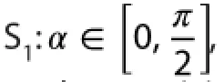
The direction of PGF （α） in S1is given by

while both of them in S2and S3are given as follows:

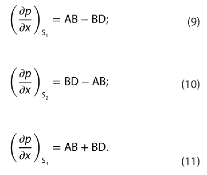
Substituting Equations （2）， （3）， （5）， and （7）/（8） into Equation（1）， we obtain the expression of PGF in S1， S2， and S3，respectively: According to Equation （11）， the expression of PGF in S3is a summation of AB and BD； namely， the PGF errors are consistently small regardless of the terrain slope. Therefore， we only investigate the PGF errors in S1and S2in the following calculation.

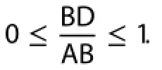
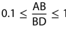
First， using Equations （5） and （6）， we calculate the proportion between the PGF2 and PGF1 in S1（BD and AB in Equation （9）） as follows:

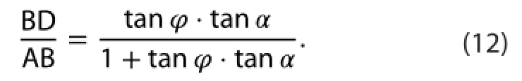
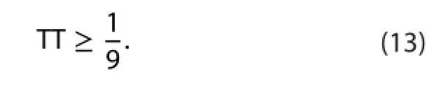
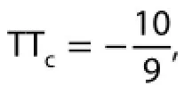
The 1/9 on the RHS of Equation （13） is the TTcin S1.

Second， using Equations （5） and （6）， we calculate the proportion between PGF2 and PGF1 in S2（AB and BD in Equation （10）） as follows:

The -10/9 on the RHS of Equation （15） is the TTcin S2. The expressions of PGF in S1， S2， and S3， and TTcin both S1and S2， are all summarized in Table 1.

In conclusion， there are three factors inducing the PGF errors of the classic method: （1） the direction of PGF （α）； （2） the slope of each vertical layer （φ）； （3） thevertical pressure gradient. The efects of α and φ can be quantifed by tan φ·tan α （Table 1）.Specifcally， when tan φ·tanor tan φ·tan α， the PGF errors of the classic method are large； and the closer α or φ is to the vertical direction， the larger the PGF errors of the classic method are.

Table 1.Expressions of PGF， TT， and PGF errors of the classic method in three situations of diferent directions of PGF.

3. Idealized experiments

In order to investigate the efects of the three factors obtained in Section 2 on inducing the PGF errors of the classic and covariant method， idealized experiments using various terrain types and pressure felds are performed. For consistency， we use the same parameters as Li， Wang， and Wang （2012）， except for the terrain and pressure felds. The basic parameters of all the experiments are introduced in Section 3.1. The experiments investigating the efects of the slope of each vertical layer and the direction of PGF are illustrated in Section 3.2. The experiments analyzing the efect of the vertical pressure gradient are demonstrated in Section 3.3.

3.1. Basic parameters

We use the central spatial discretization in the horizontal direction， and the forward scheme in the vertical direction，for the PGF of both methods. The expressions are given as follows:

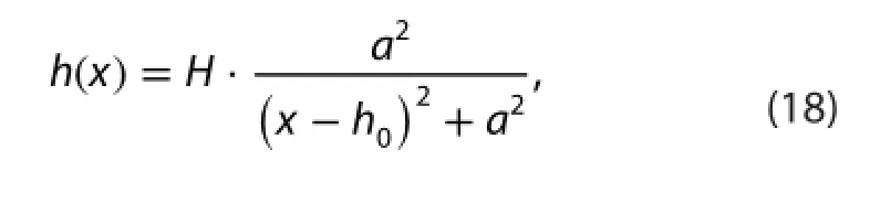
A 2D bell-shaped terrain type， is used （Figure 2）， where H is the maximum height， a = 5 km is the half width， and h0= 50 km is the middle point of the terrain. We use two types of idealized pressure felds，defned as follows （Figure 2）: （i） a pressure feld with a linear vertical pressure gradient （LP），

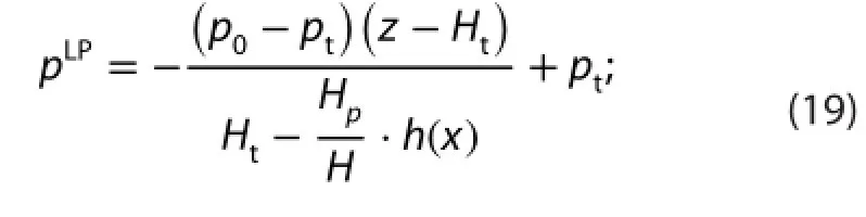
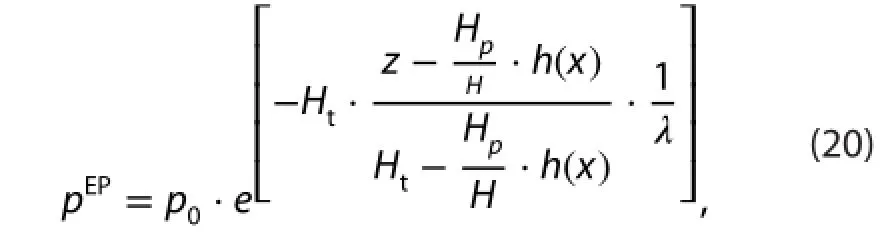
and （ii） a pressure feld with an exponential vertical pressure gradient （EP），

3.2. Effects of the direction of the PGF and slope of each vertical layer

We set H in Equation （18） from 10 to 20 km at 1-km intervals to create steep terrain， and also increase the slope of each vertical layer； and set Hpin Equation （20） from 0.5H to 1.5H km at 0.1-km intervals to obtain pressure felds with diferent directions of PGF.

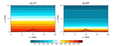
Figure 2.Pressure felds given by Equations （19） and （20）.

Figure 3.Average of PGF1 and PGF2 at diferent TT: （a） The variation of PGF1 and PGF2 according to diferent TT； （b—g） The PGF1 and PGF2 at TT = -2.728， -0.902， and -0.757， respectively.

Figure 4.REs of the PGF of the classic and covariant method: （a） The variation of REs of the two methods according to diferent TT； （b， c）The patterns of TT and RE of the classic method when the average TT is -1.247， respectively； （d， e） The patterns of TT and RE of the classic method when the average TT is -0.902， respectively.

Second， we use the experiments of H = 14 km（TTc= -1.121， closest to -10/9） as an example to further illustrate the efect of TTc. Figure 3（a） shows the variationof the average values of PGF1 and PGF2 in diferent TT. Specifcally， when TT ＜ TTc， the PGF1 and PGF2 are consistently of the same order and opposite in sign （blue and red dotted lines in Figure 3（a））， and their patterns at TT = -2.728 are shown in Figures 3（b） and （c） as an example of TT ＜ TTc. When TTc＜ TT ＜ -0.857， the PGF1 and PGF2 are still opposite in sign but no longer of the same order （e.g. the PGF1 and PGF2 at TT = -0.902 shown in Figures 3（d） and （e））. When TT ＞ -0.857 （Hp＞ H， α is in S3of Figure 1（a））， the PGF1 and PGF2 become the same in sign （e.g. the PGF1 and PGF 2 at TT = -0.757 shown in Figures 3（f） and （g））. These results verify the efects of TTcin S2and S3of Table 1.

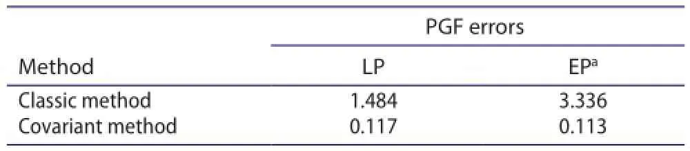
Table 2.PGF errors of the classic and covariant methods in LP and EP.

Finally， we also use the results obtained by the experiments of H = 14 km as an example to analyze the variation of the PGF errors of the classic and covariant method according to the increasing TT （Figure 4）. The pattern of TT is consistent with that of the REs of the classic method（Figures 4（b） and （c） with TT = -1.247， and Figures 4（d） and（e） with TT = -0.902）. Further， the REs of the classic method increase according to the increasing|TT|（blue line in Figure 4（a））； however， the REs of the covariant method remain almost the same （red line in Figure 4（a））. These results validate that the PGF errors of the classic method increase according to the increasing TT； whereas， the PGF errors of the covariant method are afected little by it.

3.3. Effects of vertical pressure gradient

We implement two sets of experiments to calculate the PGF of the classic and covariant method using LP and EP. Also， we set H = 4 km in Equation （18） and Hp= 0.3 km in Equations （19） and （20） to consistently compare with the results of the experiments implemented by Li， Wang， and Wang （2012）.

The REs of the PGF of both methods are summarized in Table 2. The REs of the classic method in EP are more than twice those in LP； however， the REs of the covariant method are approximately the same in EP and LP. This reveals that the exponential vertical pressure gradient is a factor inducing the PGF errors of the classic method， but not for the covariant method.

In conclusion， the three factors inducing the PGF errors of the classic method obtained by the geometric analysis in Section 2 are all validated by the idealized experiments；whereas， none of them has the efect of inducing the PGF errors of the covariant method.

4. Conclusion and discussion

This study investigates the factors inducing the PGF errors of the classic and covariant method through geometric analysis and idealized experiments. Three factors are found that induce the PGF errors of the classic method， including the direction of PGF （α）， the slope of each vertical layer （φ），and the vertical pressure gradient； however， none of them induces the PGF errors of the covariant method. Moreover，the efects of α and φ can be quantifed by tan φ·tan α（Table 1）.

The geometric analysis frst demonstrates that the terrain slope and the vertical pressure gradient can induce the PGF errors of the classic method. Then， the efect of terrain slope is generalized into the efect of the slope of each vertical layer （φ）. More importantly， a new factor， thedirection of PGF （α）， is proposed. When tanφ·tanα or tanφ·tanα， the two terms of PGF of the classic method are of the same order and opposite in sign. Subsequently， the PGF errors of the classic method are large （Table 1）， and the closer the α or φ is to the vertical direction， the larger the PGF errors of the classic method are.

The efects of all of the three factors on inducing the PGF errors of the classic method are validated by a series of idealizedexperiments. Results frst verify the analytical value of， proposed by the geometric analysis，as well as its efect on inducing the PGF errors of the classic method （Figure 3）. It is then found that the PGF errors of the classic method increase according to increasing|TT|，and their patterns are also consistent （Figure 4）. Finally，results using LP and EP validate that EP can signifcantly increase the PGF errors of the classic method （Table 2）. Moreover， all the idealized experiments demonstrate that the PGF errors of the covariant method are afected little by the three factors. Note that the comparison of the factors inducing the PGF errors of the classic and covariant methods in this study only considers the PGF term； the true beneft of the covariant method needs to be investigated using the equations of the classic and covariant methods in their entirety.

In addition， the diference between the analytical TTcand the TTcobtained in the idealized experiments may be due to using the average TT of all the grids. Further analyses need to be carried out to use the average TT of selected grids， in which PGF1 and PGF2 are of the same order. Besides， the three factors tested by the idealized pressure felds in this study are simultaneously changeddue to the analytical expression of pressure， Equation （20）. And， only the efects of TTcin S2and S3can be tested by this kind of pressure feld. Sensitivity experiments using a discrete pressure feld， in which each factor can be independently changed， are needed to further investigate the efects of these three factors. Furthermore， experiments using the real pressure feld are needed to verify the efect of TTc.

Disclosure statement

No potential confict of interest was reported by the authors.

Funding

This work was jointly supported by the National Basic Research Program of China ［973 Program， grant number 2015CB954102］；National Natural Science Foundation of China ［grant numbers 41305095 and 41175064］.

Notes on contributor

LI Jin-Xi is a PhD candidate at LASG， Institute of Atmospheric Physics， Chinese Academy of Sciences. His main research interests focus on dynamical core of atmospheric models. Recent publications include papers in Geoscientifc Model Development，Atmospheric Science Letters， and Chinese Science Bulletin.

References

Blumberg， A. F.， and G. L. Mellor. 1987. “A Description of a Three-Dimensional Coastal Ocean Circulation Model.”Paper presented at the annual meeting for the American Geophysical Union， Washington， DC， 1—16.

Corby， G. A.， A. Gilchrist， and R. L. Newson. 1972. “A General Circulation Model of the Atmosphere Suitable for Long Period Integrations.” Quarterly Journal of the Royal Meteorological Society 98: 809—832. doi:10.1002/qj.49709841808.

Gal-Chen， T.， and R. C. J. Somerville. 1975. “On the Use of a Coordinate Transformation for the Solution of the Navier-Stokes Equations.” Journal of Computational Physics 17: 209—228. doi:10.1016/0021-9991（75）90037-6.

Haney， R. L. 1991. “On the Pressure Gradient Force over Steep Topography in Sigma Coordinate Ocean Models.” Journal of Physical Oceanography 21: 610—619. doi:10.1175/1520-0485（1991）021＜0610:OTPGFO＞2.0.CO；2.

Klemp， J. B. 2011. “A Terrain-following Coordinate with Smoothed Coordinate Surfaces.” Monthly Weather Review 139: 2163—2169. doi:10.1175/MWR-D-10-05046.1.

Li， J.， Y. Li， and B. Wang. 2015. “Pressure Gradient Errors in a Covariant Method of Implementing σ-Coordinate: Idealized Experiments and Geometric Analysis.” Atmospheric and Oceanic Science Letters. （Under review）.

Li， Y. Y.， D. H. Wang， and B. Wang. 2012. “A New Approach to Implement Sigma Coordinate in a Numerical Model.”Communications in Computational Physics 12: 1033—1050. doi:10.4208/cicp.030311.230911a.

Li， Y. Y.， B. Wang， D. H. Wang， J. X. Li， and L. Dong. 2014. “An Orthogonal Terrain-following Coordinate and Its Preliminary Tests Using 2-D Idealized Advection Experiments.”Geoscientifc Model Development 7: 1767—1778. doi:10.5194/ gmd-7-1767-2014.

Lin， S. J. 1997. “A Finite-Volume Integration Method for Computing Pressure Gradient Force in General Vertical Coordinates.” Quarterly Journal of the Royal Meteorological Society 123: 1749—1762. doi:10.1002/qj.49712354214.

Ly， L. N.， and L. Jiang. 1999. “Horizontal Pressure Gradient Errors of the Monterey Bay Sigma Coordinate Ocean Model with Various Grids.” Journal of Oceanography 55: 87—97. doi:10.102 3/A:1007865223735.

Mahrer， Y. 1984. “An Improved Numerical Approximation of the Horizontal Gradients in a Terrain-following Coordinate System.” Monthly Weather Review 112 （5）: 918—922. doi:10.1175/1520-0493（1984）112＜0918:AINAOT＞2.0.CO；2.

Phillips， N. A. 1957. “A Coordinate System Having Some Special Advantages for Numerical Forecasting.” Journal of Meteorology 14: 184—185. doi:10.1175/1520-0469（1957）014＜0184:ACSHS S＞2.0.CO；2.

Qian， Y. F.， and Z. Zhong. 1986. “General Forms of Dynamic Equations for Atmosphere in Numerical Models with Topography.” Advances in Atmospheric Sciences 3: 10—22. doi:10.1007/BF02680042.

Qian， Y. F.， and T. J. Zhou. 1994. “Error Subtraction Method in Computing Pressure Gradient Force for High and Steep Topographic Areas.” Journal of Tropical Meteorology 10: 358—368. Shchepetkin， A. F.， and J. C. McWilliams. 2003. “A Method for Computing Horizontal Pressure-gradient Force in an Oceanic Model with a Nonaligned Vertical Coordinate.”Journal of Geophysical Research 108: 3090—3123. doi:10.1029/2001JC001047.

Smagorinsky， J.， R. F. Strickler， W. E. Sangster， S. Manabe， J. L. Halloway Jr. and G. D. Hembree. 1967. “Prediction Experiments with a General Circulation Model.” Paper presented at Dynamics of Large Scale Atmospheric Processes， Moscow， USSR， 70—134.

Yan， H.， and Y. F. Qian. 1981. “On the Problems in the Coordinate Transformation and the Calculation of the Pressure Gradient Force in the Numerical Models with Topography.” Chinese Journal of Atmospheric Sciences 5: 175—187. doi:10.3878/j. issn.1006-9895.1981.02.07.

Yoshio， K. 1968. “Note on Finite Diference Expressions for the Hydrostatic Relation and Pressure Gradient Force.”Monthly Weather Review 96 （9）: 654—656. doi:10.1175/1520-0493（1968）096＜0654:NOFDEF＞2.0.CO；2.

Zeng， Q. C. 1979. “Basic Equations and Coordinate Transformation.”Mathematical and Physical Fundamental Theory for Numerical Weather Prediction. Vol. 1， 22—25. Beijing: Science Press.

Zeng， X. P.， and Z. H. Ren. 1995. “Quantitative Analysis of the Discretization Errors of the Horizontal Pressure Gradient Force over Sloping Terrain.” Chinese Journal of Atmospheric Sciences 19: 722—732. doi:10.3878/j.issn.1006-9895.1995.06.09.

地形追随坐标系； 气压梯度力误差； 垂直气压梯度； 气压梯度方向； 垂直层坡度

31 December 2015

CONTACT LI Yi-Yuan liyiyuan@mail.iap.ac.cn

© 2016 The Author（s）. Published by Taylor & Francis.

This is an Open Access article distributed under the terms of the Creative Commons Attribution License （http://creativecommons.org/licenses/by/4.0/）， which permits unrestricted use， distribution， and reproduction in any medium， provided the original work is properly cited.