CAO Ning ， REN Bao-Hua ， ZHENG Jian-Qiu and XU Di

School of Earth and Space Sciences， University of Science and Technology of China， Hefei， China

Evaluation of the surface heat budget over the tropical Indian Ocean in two versions of FGOALS

CAO Ning ， REN Bao-Hua ， ZHENG Jian-Qiu and XU Di

School of Earth and Space Sciences， University of Science and Technology of China， Hefei， China

Changes of the net ocean surface heat fux （Qnet） into the tropical Indian Ocean （TIO） may be an indicator of the climate changes in the Asia and Indian-Pacifc Ocean regions with the steadily warming trend in the TIO since the 1950s. Using two observational ocean surface fux products，this letter evaluates the historical simulations of Qnetover the TIO during 1984-2005 in two versions of FGOALS， from CMIP5. The results show that both models present a basin-wide underestimation of net surface heat fux， possibly resulting from the positive latent heat fux biases extending over almost the entire TIO basin. Both models share an Indian Ocean dipole-like bias in the net surface heat fux， consistent with precipitation， SST， and subsurface ocean temperature biases， which can be traced to errors in the South Asian summer monsoon. Area-averaged annual time series analyses of the surface heat budget imply that the FGOALS-s2 bias lies more in radiative imbalance， illustrating the need to improve cloud simulation； while the FGOALS-g2 bias presents ocean surface turbulence fux as the key process， requiring improvement in the simulation of oceanic processes. Neither FGOALS-g2 nor FGOALS-s2 can capture the decreasing tendency of Qnetwell. All observed and simulated datasets imply surface latent heat fux as the primary contributing component， indicating the simulation biases of models may derive mainly from the biases in simulating latent heat fux. A small latent heat fux increase in models can be considered to be slowed by relaxed wind， increased stability， and surface relative humidity.

ARTICLE HISTORY

Accepted 10 May 2016

Tropical Indian Ocean； heat budget analysis； climatology；trend； FGOALS

热带印度洋海表热收支平衡极大地影响着周边的气候变化，对此的精确模拟是提高海气耦合模式模拟区域气候能力的重要一方面。本文使用不同数据来源的格点资料集OAFlux和NOCS-V2的海表通量产品，评估了FGOALS-g2和FGOALS-s2两个模式对热带印度洋海表热收支平衡的模拟结果。发现模拟净热通量存在海盆尺度的低估，来源于潜热通量的高估。相对而言FGOALS-s2模拟的辐射通量误差更大。模式无法模拟出净热通量的减少趋势，主因在于对潜热通量趋势模拟能力不足。

1. Introduction

Earth’s energy balance is controlled by the incoming solar radiation and the outgoing thermal radiation. Climate changes may derive from an imbalance in global energy. Oceans play a key role in the climate system， partly because of their large heat-holding capacity. Deser et al. （2010） indicated that only 3.5 m of water can hold as much energy as the total column air. Energy in the oceans not only drives ocean circulation， but also-after moving from ocean to atmosphere via evaporation cooling， sensible heat fux，and longwave radiation-then drives atmospheric circulation （Trenberth， Fasullo， and Kiehl 2009）.

The oceanic heat budget has attracted considerable attention among climate scientists， generating much scientifc discussion （e.g. Moisan and Niiler 1998； Trenberth， Fasullo， and Kiehl 2009； Trenberth and Fasullo 2010）. The Indian Ocean （IO） is the third largest of the world’s oceans，covering about 20% of Earth’s water surface. The diferential heating between the land mass and adjacent ocean results in the strongest tropical monsoon system； namely，the South Asia monsoon， or Indian monsoon. Studying the IO’s heat budget changes can provide us with a better understanding of the changes in the Asian monsoon systems. The tropical Indian Ocean （TIO） has been showing a signifcant basin-scale warming trend since the 1950s（Giannini， Saravanan， and Chang 2003； Hoerling and Kumar 2003； Hoerling et al. 2004）， and this warming trend has been detected and discussed using climate models（Du and Xie 2008； Dong， Zhou， and Wu 2014； Dong and Zhou 2014； Li， Xie， and Du forthcoming； Zheng et al. 2016）.Alory and Meyers （2009） ascribed the IO’s surface warming mainly to a decrease in upwelling related to the slowing of wind-driven Ekman pumping.

Climate models face a number of challenges， but one of the more prominent issues is their large underestimation of surface fux imbalance （IPCC 2007）. Two versions of once such model-the grid-point and spectral versions of FGOALS， developed with considerable ongoing efort at the LASG， IAP， Chinese Academy of Sciences-are no exception in this respect. Dong and Zhou （2014） investigated the IO’s warming mechanisms in version 2 of the grid-point and spectral versions of FGOALS and stated that in both models it is mainly caused by atmospheric forcing via radiative and turbulent fuxes. Net ocean-surface heat fux （Qnet）， as a result of the radiation and turbulence heat budget， can refect the level of surface heat imbalance. Rahul and Gnanaseelan （2013） investigated the decreasing trend of Qnetin the TIO， and suggested that radiation imbalance plays a secondary role relative to changing oceanic processes， which are mainly responsible for the IO’s warming trend.

However， the performance of FGOALS in simulating the ocean surface heat budget over the TIO， as well as the related bias sources， remains unclear. Version 2 of the gridpoint and spectral versions of FGOALS were chosen for this study because of their continuous improvements in many aspects of model performance. The models have been involved in various model intercomparison projects and subjected to numerous evaluations and analyses， especially in the joining areas of Asia and the Indian-Pacifc Ocean （see Zhou et al. （2014） for a summary）. On the other hand， the FGOALS models have also been widely used for climate predictions and projections over East Asia. It is therefore important to study the model biases in representing the ocean surface heat budget and related physical processes over the TIO， for improving regional climate predictions and projections.

This study aims to detect the changes and trends of Qnetand evaluate （against observation） the historical simulations with regard to the ocean surface heat budget over the TIO in the two models of FGOALS version 2. Section 2 presents the models， data， and method. In Section 3，the results are evaluated and the related bias sources discussed with respect to the climatology， annual variability，and trend of Qnet. Section 4 provides a brief summary of the key fndings.

2. Model， data， and method

The grid-point and spectral versions of FGOALS （both version 2； FGOALS-g2 and FGOALS-s2， respectively） are the latest versions of the model developed by researchers mainly working at LASG， IAP， and have participated in CMIP5. They both include four individual components: atmosphere， ocean， land， and sea-ice components， using LICOM2.0 as the oceanic component； the atmospheric components are GAMIL2.0 for FGOALS-g2 and SAMIL2.0 for FGOALS-s2 （more details available in Li et al. （2013） and Bao et al. （2013））.

The OAFlux data-set （Yu and Weller 2007） is provided by the Woods Hole Oceanographic Institution OAFlux project（http://oafux.whoi.edu）. The turbulence heat fux data in this data-set are combined with numerical weather prediction reanalysis and satellite observations using an objective analysis method. The ocean surface radiation products（including shortwave radiation and longwave radiation）are directly adapted from the ISCCP data-set （Zhang et al. 2004）. Yu， Jin， and Weller （2007） compared several heat fux products and concluded that OAFlux+ISCCP matches better with observations from ships and buoys over the IO. The National Oceanography Centre Southampton （NOCS）Version 2.0 Surface Flux Data-set， constructed using optimal interpolation by the in situ ship observations from ICOADS （Berry and Kent 2011）， is used as another observational data-set. These two datasets have independent data sources and quite diferent analysis methods.

In general， the Qnetinto oceans can be computed from radiation heat fuxes and turbulence heat fuxes by the following equation:

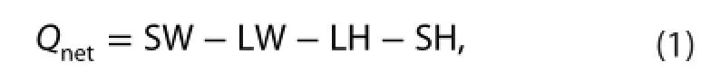
where SW and LW are net downward shortwave radiation and upward longwave radiation， respectively， and LH and SH are upward latent heat fux and sensible heat fux，respectively.

3. Results

3.1. Climatology

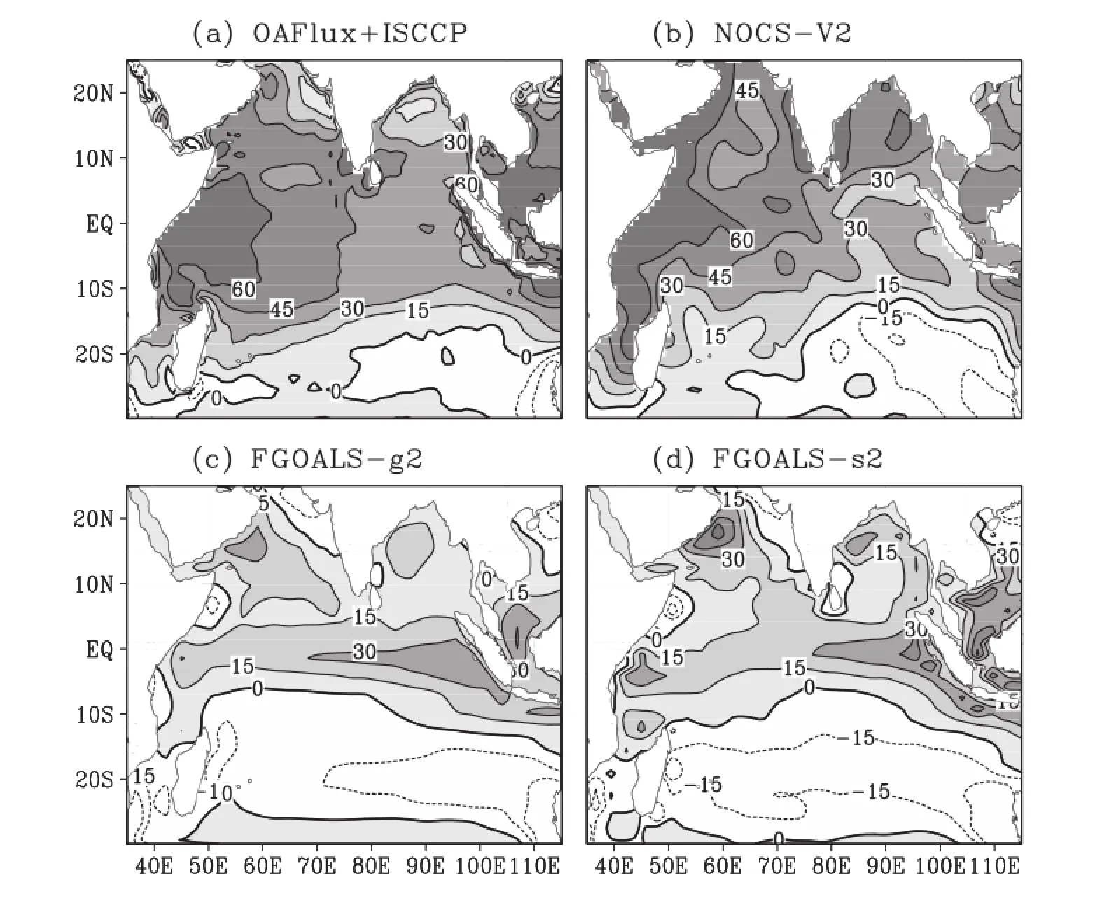
Figure 1. The climatological mean Qnetin the IO captured by the observational （OAFlux+ISCCP and NOCS-V2） and model-simulated（FGOALS-g2 and FGOALS-s2） datasets for the period 1984-2005.

Figure 1 presents the climatological mean Qnetinto the TIO（30°S-25°N， 35-115°E） using the two observational datasets of OAFlux+ISCCP and NOCS-V2， and the two model-simulated datasets of FGOALS-g2 and FGOALS-s2， for the present study period of 1984-2005. It is evident that both the observed and model-simulated datasets characterize the pattern of heat gain in the northern tropical IO and heat loss in the southern tropical IO. However， the amplitude of heat gain according to the observational datasets is much larger than that according to the model-simulated datasets. The overall amplitude bias （underestimation） of the models is approximately 30 W m-2，resulting in the zero line of Qnetin the two models being about 10° north of that observed. The largest heat loss occurs in the southeastern tropical IO， of the west coast of Australia， which is captured by all the observed and model-simulated datasets. However， the largest observed heat gain， occurring over the northwestern tropical IO， of the east coast of Africa and the Middle East coast， is not reproduced by the two models. Relatively， the large heat gain observed in the South China Sea and Indonesian regions can be fairly well reproduced by the models. Pattern correlation coefcients between the observed and simulated datasets in presenting the climatology of Qnetover the TIO are computed using the centered pattern correlation method （Santer， Wigley， and Jones 1993）. The results show that the two observed datasets correlate with a coefcient of 0.76， and the model simulation of FGOALS-g2 （FGOALS-s2） correlates to the observations of OAFlux+ISCCP and NOCS-V2 with coefcients of 0.60 and 0.55 （0.63 and 0.63）， respectively. Therefore， the two versions of FGOALS2 capture the basic characteristics of climatological mean Qnetover the TIO during 1984-2005 reasonably well.

In particular， both versions of FGOALS share an IOD-like（IOD: Indian Ocean dipole） bias in the net surface heat fux. Actually， physically consistent biases in precipitation， SST，and subsurface ocean temperature， with a strong easterly wind bias along the equatorial IO， which resemble the IOD mode of interannual variability in nature， are common in these two versions of FGOALS （fgure not shown）， and most CMIP5 climate models （Li， Xie， and Du 2015a）. Li， Xie，and Du （2015a， 2015b） traced such IOD-like biases back to errors in the South Asian summer monsoon. Thus， improving the monsoon simulation is a priority and would lead to better regional climate simulations in the ocean surface heat budget and related physical processes over the TIO.

Figure 2 presents the models biases of relevant components including SW， LW， LH， and SH， against the results of OAFlux+ISCCP data. It is evident that the basin-wide underestimation of Qnetmay come from the positive LH biases extending over almost the entire TIO region， especially in FGOALS-s2， whose sensitivity to greenhouse gas forcing is greater than in most CMIP5 models （Chen， Zhou，and Guo 2014）. This is very diferent from most CMIP5 models. Actually， Li and Xie （2012， 2014） identifed the tropical-wide biases in SST and surface heat fuxes and traced them back to a common overestimation of tropical cloud in coupled models that can refect incoming solar shortwave radiation and thus result in negative surface SW bias.

3.2. Interannual variability

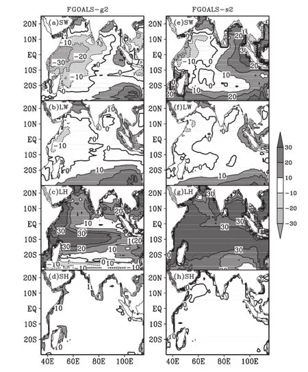
Figure 2. The simulated biases of SW， LW， LH， and SH in （a-d） FGOALS-g2 and （e-h） FGOALS-s2.

The time series of Qnetaveraged over the TIO during 1984-2005 from the observed and simulated datasets are shown in Figure 3， together with time series of related surface heat fux components including SW， LW， LH， and SH. On an annual average basis， over the TIO， both observational datasets show an approximate 30 W m-2yr-1heat gain，but the simulated heat gain is almost zero， with values mostly below 5 W m-2. Analysis of the annual cycle shows that， in observations， two （June and July） out of twelve months in a complete year lose heat； whereas in simulations， four （May， June， July and August） out of twelve months in a complete year lose heat. These diferences may partly explain the underestimation of simulated Qneton the interannual scale. The OAFlux+ISCCP Qnetpresents a relatively steady series with interdecadal variability from 1984 to 2001； however， there is an abrupt decline after 2001， which has been suggested to be a nonphysical change-afected by satellite cloud viewing geometry artifacts， as well as errors in ancillary datasets （Evan，Heidinger， and Vimont 2007； Raschke， Bakan， and Kinne 2006）. Despite these uncertainties， the Qnetvariability undoubtedly results from variabilities of turbulent and radiative heat fux components. The two observational datasets and FGOALS-g2 show good agreement in terms of SW estimates， but FGOALS-s2 shows an overestimation of about 6 W m-2relative to ISCCP. Previous assessments of FGOALS-s2 show that overestimated SW along the eastern coast of the Pacifc and Atlantic oceans， which is related to the warm biases in these regions， is due to the underestimation of low-level cloud （Lin， Yu， and Liu 2013）. The ISCCP data-set gives a decadal-scale variability in LW，which seems akin to nonphysical changes， while NOCS-V2 and the two models show steady states； although， there are overestimations of approximately 15 W m-2in both models relative to NOCS-V2. For LH， both OAFlux and NOCS-V2 show an increasing trend during 1984-1999 and a weak decreasing trend during 1999-2005. The simulations of FGOALS-g2 and FGOALS-s2， however， produce overestimations of about 13 W m-2and 30 W m-2relative to OAFlux. NOCS-V2 is 10 W m-2larger than OAFlux in estimating LH. For SH， FGOALS-s2 agrees well with both observational datasets， except small underestimations and the non-reproduction of an observed increasing trend， but FGOALS-g2 shows large overestimations of about 7 W m-2relative to OAFlux. These biases of the two models in simulating the surface heat fux components ultimately resultin large underestimations in simulating the heat gain of the TIO. It is notable that the FGOALS-s2 bias mainly lies in the overestimations of SW and LH， while the FGOALS-g2 bias mainly lies in the overestimation of turbulence heat fux， including latent and sensible heat fuxes.

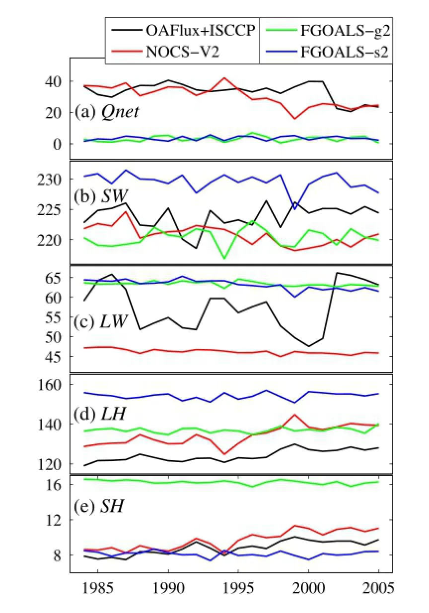
Figure 3. Time series of Qnetand related heat fux component （SW，LW， LH， and SH） averaged over the TIO from the observational and simulated datasets.

The statistical relationship between the Qnettemporal variability and that of heat fux components is computed（not shown）. Generally， NOCS-V2 indicates LH as the primary contributor of Qnetvariability. However， the Qnetvariability in OAFlux+ISCCP is greatly infuenced by the variability of LW， which may be non-physical. For the models，both FGOALS-s2 and FGOALS-g2 present LH as the primary contributor of Qnetvariability， with nearly the same correlation coefcient； however， FGOALS-g2 presents a much smaller variance contribution than FGOALS-s2， and the contrary SW in FGOALS-g2 shows an almost equal infuence as LH for both correlation and variance contributions. Other components make relatively small contributions to the variability of Qnet， with either weak correlations or small variance contributions. Nevertheless， it is the LH trend that primarily determines the trend of Qnetfor both observations and model simulations.

3.3. Trend

Using time series of net surface heat fux averaged over the TIO during 1984-2005 from the observational and simulated datasets shown in Figure 3， the trends of Qnetand related heat fux components are computed by linear least-squares ftting and presented in Table 1. In the observational datasets， the net surface heat fux change during 1984-2005 shows a signifcant decreasing tendency over the TIO， and there is a signifcant increase in LH and SH that contributes primarily to the decreased Qnet. In the simulated results of the FGOALS models， however， there is no signifcant trend， and the computed trend amplitudes are far below the detection limit of observations （Yu， Jin， and Weller 2007）， consistent with results of previous studies performed using CMIP3 climate models （Du and Xie 2008）. In terms of spatial patterns， the trends of Qnetover the TIO during 1984-2005 determined using the two observational and two simulated datasets are shown in Figure 4. The OAFlux+ISCCP data-set shows a distinct negative trend in the central TIO and very weak trends in surrounding regions， while the NOCS-V2 data-set presents a basinwide negative trend. Given the fact that the OAFlux+ISCCP data-set may feature a non-physical abrupt decline in 2001， the 1984-2000 Qnettrend for the OAFlux+ISCCP data-set is also computed （not shown）， and the pattern is similar to the 1984-2005 trend， except with smaller amplitude. A robust feature of the observations is the maximum decrease in the equatorial central TIO. These results mean that the net heat into the TIO is generally decreasing from the 1980s through to the early 2000s， consistent with previous studies （Schott， Xie， and McCreary 2009； Rahul and Gnanaseelan 2013）. The trend patterns of net heat fux produced by the FGOALS models do not show an identifable trend， which is consistent with the TIO feld mean trends. To investigate the contributions of surface heat fux components to the Qnettrends in diferent datasets， a Taylor diagram （Figure 5） is produced to show how thesecomponent trends match the Qnettrends with pattern statistics. Signifcantly， all the observational and simulated datasets present LH as the primary contributing component. The NOCS-V2 data-set is the most obvious， and the LHs in OAFlux+ISCCP and FGOALS-s2 have the same correlation coefcient with their respective Qnettrend， but FGOALS-s2 simulates a larger variance contribution to Qnet. Meanwhile， the LHs in OAFlux+ISCCP and FGOALS-g2 show the same variance contribution to Qnet， but FGOALS-g2 has a weaker correlation. Other components show either tooweak a correlation or too small a variance contribution to Qnetin both the observational and simulated datasets. These results show that the biases of FGOALS-g2 and FGOALS-s2 in simulating the Qnettrends may derive mainly from the biases in simulating LH trends. Further evaluations of LH trend biases in models may be helpful in understanding the model-observation inconsistency. Li et al. （2011） investigated the ocean surface LH trend and suggested that the LH increase is closely associated with both the SST warming forces as direct causes， and surface wind circulation changes as indirect factors. A recent study by Cao， Ren， and Zheng （2015） shows that trends of LH-related SST （i.e. ocean surface warming） and air specifc humidity are grossly overestimated over the Pacifc. Du and Xie （2008） suggested that relaxed wind，increased stability， and relative humidity slow the rate of latent heat fux increase.

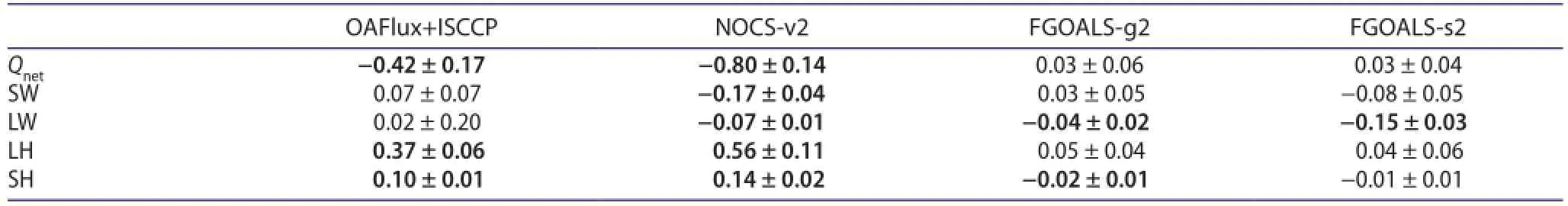
Table 1. The linear trends and 95% confdence levels of net surface heat fux （Qnet） and related heat fux components.

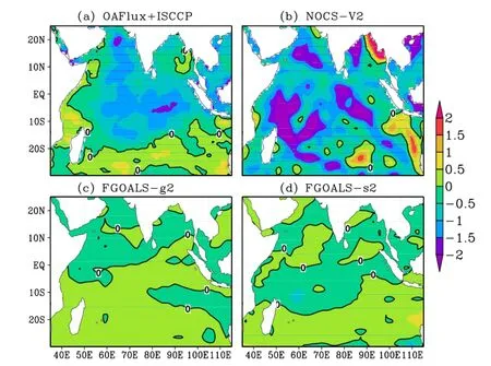
Figure 4. Trends of Qnetover the TIO during 1984-2005 determined observationally by （a） OAFlux+ISCCP and （b） NOCS-V2， and simulated by （c） FGOALS-g2 and （d） FGOALS-s2.

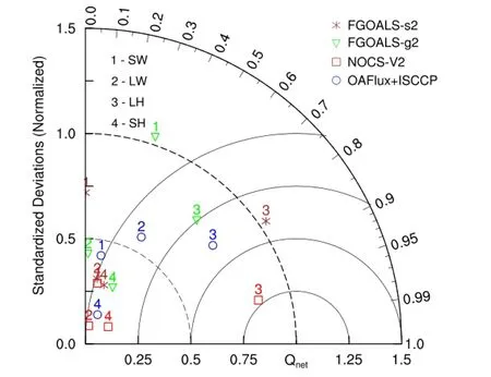
Figure 5. Taylor diagram showing how the trends of ocean surface heat fux components （SW， LW， LH， and SH） contribute to the trend of Qnetover the TIO during 1984-2005， determined by the two observational datasets （OAFlux+ISCCP and NOCS-V2） and two simulated datasets （FGOALS-g2 and FGOALS-s2）.

4. Summary

Using two independent observational ocean surface heat fux products （OAFlux+ISCCP and NOCS-V2）， the characteristics of the climatology， annual variability and trend of Qnetsimulated by two versions of FGOALS over the TIO during 1984-2005 are assessed in this paper， and the related possible causes of model biases discussed.

For the mean state， despite the uncertainties of observations， both models present a basin-wide underestimation of approximately 30 W m-2， resulting in the zero line of Qnetin the models being about 10° north of that observed. Surface latent heat fux， which is largely overestimated over almost the entire TIO region， is considered to be the most likely source of this basin-scale underestimation of Qnet，especially in FGOALS-s2， whose sensitivity to greenhouse gas forcing is greater than that in most CMIP5 models. Besides， both models share an IOD-like bias in net surface heat fux. Physically consistent biases in precipitation， SST，and subsurface ocean temperature with a strong easterly wind bias along the equatorial IO， which resemble the IOD mode of interannual variability in nature， are common in these two versions of FGOALS， and most CMIP5 climate models. Li， Xie， and Du （2015a， 2015b） traced such IOD-like biases back to errors in the South Asian summer monsoon. Thus， improving the monsoon simulation is a priority and would lead to better regional climate simulation in the ocean surface heat budget and related physical processes over the TIO.

In the annual time series of net surface heat fux averaged over the TIO， both FGOALS models indicate relatively balanced surface heat， with an approximate 0 W m-2heat fux into the ocean， which is far below the approximate 30 W m-2fux in both observational datasets. Notable features are that the FGOALS-s2 bias mainly lies in the overestimations of SW and LH， while the FGOALS-g2 bias mainly lies in the overestimation of turbulence heat fux， including latent and sensible heat fuxes. As FGOALS-s2 has a greater sensitivity to greenhouse gas forcing， the key process of the surface heat budget over the TIO is more likely the radiative imbalance， illustrating the need to improve cloud simulation. Meanwhile， FGOALS-g2 presents surface turbulence fux as the key process， though it seems to need further improvement in representing oceanic processes. A maximum decreasing tendency exists in the equatorial central TIO in both observational datasets， meaning that the net heat into the TIO shows a generally decreasing trend from the 1980s through to the early 2000s. Neither FGOALS-g2 nor FGOALS-s2 can capture this feature well. All the observational and simulated datasets imply surface latent heat fux as the primary contributing component， indicating the simulated biases of FGOALS-g2 and FGOALS-s2 may derive mainly from the biases in simulating LH. A small LH increase in models can be considered to be slowed by relaxed wind， increased stability， and surface relative humidity.

Acknowledgements

The authors would like to thank the two anonymous reviewers for their valuable and constructive comments. The authors also acknowledge the modeling groups of FGOALS， for providing their model data. The OAFlux data were provided by the Woods Hole Oceanographic Institution OAFlux project. The NOCS Version 2.0 surface fux datasets are archived at NCAR’s Computational and Information Systems Laboratory.

Disclosure statement

No potential confict of interest was reported by the authors.

Funding

This work was supported by the National Basic Research Program of China ［grant number 2012CB417403］； State Key Laboratory of Tropical Oceanography， South China Institute of Oceanology， Chinese Academy of Sciences ［project number LTO1502］.

Notes on contributors

CAO Ning is a PhD candidate at the School of Earth and Space Sciences （ESS）， University of Science and Technology of China（USTC）. His main research interests are ocean-atmosphere interaction and numerical modeling of climate. His recent publications include papers in Advances in Atmospheric Sciences，and Atmospheric and Oceanic Science Letters.

REN Bao-Hua is a professor at ESS， USTC. His main research interests are climate dynamics and atmospheric environment. His recent publications include papers in Geophysical ResearchLetters， Journal of Climate， Journal of Geophysical Research-Atmospheres， Advances in Atmospheric Sciences， Chinese Journal of Atmospheric Sciences， and other journals.

ZHENG Jian-Qiu is a lecturer at ESS， USTC. His main research interests are ocean-atmosphere interaction and East Asian monsoon. His recent publications include papers in Journal of Climate， Chinese Journal of Atmospheric Sciences， Climatic and Environmental Research， and other journals.

XU Di is a MS candidate at ESS， USTC. Her main research interest is East Asian monsoon. Her recent publications include papers in Journal of the Meteorological Sciences and other journals.

ORCID

CAO Ning http://orcid.org/0000-0001-6957-545X

References

Alory， G.， and G. Meyers. 2009. “Warming of the Upper Equatorial Indian Ocean and Changes in the Heat Budget （1960-1999）.”Journal of Climate 22: 93-113.

Bao， Q.， P. F. Lin， T. J. Zhou， Y. Liu， Y. Q. Yu， G. Wu， et al. 2013. “The Flexible Global Ocean-Atmosphere-Land System Model，Spectral Version 2: FGOALS-S2.” Advances in Atmospheric Sciences 30: 561-576.

Berry， D. I.， and E. C. Kent. 2011. “Air-Sea Fluxes from ICOADS: The Construction of a New Gridded Dataset with Uncertainty Estimates.” International Journal of Climatology 31: 987-1001. Cao， N.， B. H. Ren， and J. Q. Zheng. 2015. “Evaluation of CMIP5 Climate Models in Simulating 1979-2005 Oceanic Latent Heat Flux over the Pacifc.” Advances in Atmospheric Sciences 32: 1603-1616.

Chen， X. L.， T. J. Zhou， and Z. Guo. 2014. “Climate Sensitivities of Two Versions of FGOALS Model to Idealized Radiative Forcing.” Science China： Earth Science 57: 1363-1373.

Deser， C.， M. A. Alexander， S. P. Xie， and A. S. Phillips. 2010. “Sea Surface Temperature Variability: Patterns and Mechanisms.”Annual Review of Marine Science 2: 115-143.

Dong， L.， and T. J. Zhou. 2014. “The Indian Ocean Sea Surface Temperature Warming Simulated by CMIP5 Models during the Twentieth Century: Competing Forcing Roles of GHGs and Anthropogenic Aerosols.” Journal of Climate 27: 3348-3362.

Dong， L.， T. J. Zhou， and B. Wu. 2014. “Indian Ocean Warming during 1958-2004 Simulated by a Climate System Model and Its Mechanism.” Climate Dynamics 42: 203-217.

Du， Y.， and S. P. Xie. 2008. “Role of Atmospheric Adjustments in the Tropical Indian Ocean Warming during the 20th Century in Climate Models.” Geophysical Research Letters 35: L08712. doi:10.1029/2008GL033631.

Evan， A. T.， A. K. Heidinger， and D. J. Vimont. 2007. “Arguments against a Physical Long-term Trend in Global ISCCP Cloud Amounts.” Geophysical Research Letters 34: L04701. doi:10.1029/2006GL028083.

Giannini， A.， R. Saravanan， and P. Chang. 2003. “Oceanic Forcing of Sahel Rainfall on Interannual to Interdecadal Time Scales.”Science 302: 1027-1030.

Hoerling， M.， and A. Kumar. 2003. “The Perfect Ocean for Drought.” Science 299: 691-694.

Hoerling， M. P.， J. W. Hurrell， T. Xu， G. T. Bates， and A. S. Phillips. 2004. “Twentieth Century North Atlantic Climate Change. Part II: Understanding the Efect of Indian Ocean Warming.”Climate Dynamics 23: 391-405.

IPCC 2007. Climate Change 2007： The Physical Science Basis：Contribution of Working Group I to the Fourth Assessment Report of the Intergovernmental Panel on Climate Change，edited by S. Solomon， et al， 996. Cambridge: Cambridge University Press.

Li， G.， and S. P. Xie. 2012. “Origins of Tropical-wide SST Biases in CMIP Multi-model Ensembles.” Geophysical Research Letters 39: L22703. doi:http://dx.doi.org/10.1029/2012GL053777.

Li， G.， and S. P. Xie. 2014. “Tropical Biases in CMIP5 Multimodel Ensemble: The Excessive Equatorial Pacifc Cold Tongue and Double ITCZ Problems.” Journal of Climate 27: 1765-1780.

Li， G.， B. Ren， C. Yang， and J. Zheng. 2011. “Revisiting the Trend of the Tropical and Subtropical Pacifc Surface Latent Heat Flux during 1977-2006.” Journal of Geophysical Research 116: D10115. doi:10.1029/2010JD015444.

Li， L. J.， P. F. Lin， Y. Q. Yu， B. Wang， T. J. Zhou， L. Liu， J. P. Liu， et al. 2013. “The Flexible Global Ocean-Atmosphere-Land System Model， Grid-Point Version 2: FGOALS-G2.” Advances in Atmospheric Sciences 30: 543-560.

Li， G.， S. P. Xie， and Y. Du. 2015a. “Monsoon-Induced Biases of Climate Models over the Tropical Indian Ocean.” Journal of Climate 28: 3058-3072.

Li， G.， S. P. Xie， and Y. Du. 2015b. “Climate Model Errors over the South Indian Ocean Thermocline Dome and Their Efect on the Basin Mode of Interannual Variability.” Journal of Climate 28: 3093-3098.

Li， G.， S. P. Xie， and Y. Du. forthcoming. “A Robust but Spurious Pattern of Climate Change in Model Projections over the Tropical Indian Ocean.” Journal of Climate. doi:10.1175/ JCLI-D-15-0565.1.

Lin， P. F.， Y. Q. Yu， and H. L. Liu. 2013. “Long-term Stability and Oceanic Mean State Simulated by the Coupled Model FGOALS-S2.” Advances in Atmospheric Sciences 30: 175-192.

Moisan， J. R.， and P. P. Niiler. 1998. “The Seasonal Heat Budget of the North Pacifc: Net Heat Flux and Heat Storage Rates（1950-1990）.” Journal of Physical Oceanography 28: 401-421.

Rahul， S.， and C. Gnanaseelan. 2013. “Net Heat Flux over the Indian Ocean: Trends， Driving Mechanisms， and Uncertainties.” Geoscience and Remote Sensing Letters， IEEE 10: 776-780.

Raschke， E.， S. Bakan， and S. Kinne. 2006. “An Assessment of Radiation Budget Data Provided by the ISCCP and GEWEXSRB.” Geophysical Research Letters 33 （L07812）: 2005G. doi:10.1029/L025503.

Santer， B. D.， T. M. L. Wigley， and P. D. Jones. 1993. “Correlation Methods in Fingerprint Detection Studies.” Climate Dynamics 8: 265-276.

Schott， F. A.， S. P. Xie， and J. P. McCreary. 2009. “Indian Ocean Circulation and Climate Variability.” Reviews of Geophysics 47: RG1002.

Trenberth， K. E.， and J. T. Fasullo. 2010. “An Observational Estimate of Inferred Ocean Energy Divergence.” Journal of Physical Oceanography 38: 984-999.

Trenberth， K. E.， J. T. Fasullo， and J. Kiehl. 2009. “Earth’s Global Energy Budget.” Bulletin of the American Meteorological Society 90: 311-323.

Yu， L. S.， and R. A. Weller. 2007. “Objectively analyzed air-sea heat fuxes （OAFlux） for the global oceans.” Bulletin of the American Meteorological Society 88: 527-539.

Yu， L. S.， X. Jin， and R. A. Weller. 2007. “Annual， Seasonal， and Interannual Variability of Air-Sea Heat Fluxes in the Indian Ocean.” Journal of Climate 20: 3190-3209.

Zhang， Y. C.， W. B. Rossow， A. A. Lacis， V. Oinas， and M. I. Mishchenko. 2004. “Calculation of Radiative Fluxes from the Surface to Top of Atmosphere Based on ISCCP and Other Global Data Sets: Refnements of the Radiative Transfer Model and the Input Data.” Journal of Geophysical Research 109: D19105.

Zheng， X. T.， L. Gao， G. Li， and Y. Du. 2016. “The Southwest Indian Ocean Thermocline Dome in CMIP5 Models: Historical Simulation and Future Projection.” Advances in Atmospheric Sciences 33: 489-503.

Zhou， T. J.， Y. Q. Yu， Y. M. Liu， and B. Wang. 2014. Flexible Global Ocean-Atmosphere-Land System Model. Heidelberg: Springer，483. doi:10.1007/978-3-642-41801-3.

净热通量； 热收支； 热带印度洋； FGOALS 模式

16 March 2016 Revised 21 April 2016

CONTACT REN Bao-Hua ren@ustc.edu.cn

© 2016 The Author（s）. Published by Informa UK Limited， trading as Taylor & Francis Group.

This is an Open Access article distributed under the terms of the Creative Commons Attribution License （http://creativecommons.org/licenses/by/4.0/）， which permits unrestricted use， distribution， and reproduction in any medium， provided the original work is properly cited.