Zhong WANG（王忠）Shangbin CUI（崔尚斌）

Department of Mathematics，Sun Yat-Sen University，Guangzhou 510275，China

E-mail∶wangzh79@mail2.sysu.edu.cn；cuishb@mail.sysu.edu.cn



ON THE CAUCHY PROBLEM OF A COHERENTLY COUPLED SCHRüODINGER SYSTEM∗

Zhong WANG（王忠）Shangbin CUI（崔尚斌）

Department of Mathematics，Sun Yat-Sen University，Guangzhou 510275，China

E-mail∶wangzh79@mail2.sysu.edu.cn；cuishb@mail.sysu.edu.cn

In this article，we consider the well-posedness of a coherently coupled Schrüodinger system with four waves mixing in space dimension n≤4.The Cauchy problem for the cubic system is studied in L2for n≤2 and in H1for n≤4.We obtain two sharp conditions between global existence and blow up.

Cauchy problem；coherently；Schrüodinger system；global existence

2010 MR Subject Classification35A05；35B65

1　Introduction

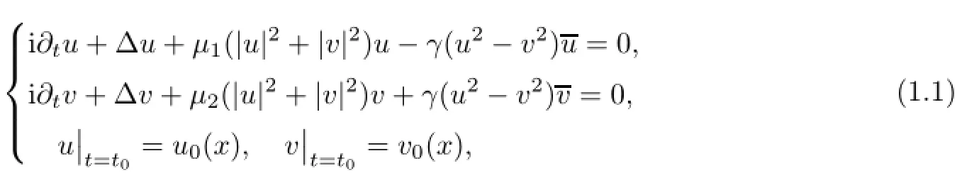
In this article，we consider the Cauchy problem of the following nonlinear Schrüodinger system where u and v are complex-valued function of（t，x）∈R×Rn，n≤4，△is the Laplacian in Rn，andµ1，µ2，γ are real constants.This type of systems describes the propagation of orthogonally polarized waveguide modes in the Kerr-type nonlinear medium，and widely arises in many physical fields，for instance，in nonlinear optics，Bose-Einstein condensates，plasma physics；see［1，6，13，14］.In the case γ=0，the system is called incoherently coupled nonlinear Schrüodinger equations（ICNLS），and in the case γ 6=0，it is referred to as coherently coupled nonlinear Schrüodinger equations（CCNLS）［6，7，13］.In the CCNLS case γ 6=0，the terms u2¯v and v2¯u correspond to the four wave mixing process，which arises due to the coherent coupling between the co-propagating fields，cf.［6，7，13］.For more details of the physical background of the above equations，we refer the reader to see the references mentioned above.

Moreover，we give now an example.When n=µ1=µ2=1，γ=0，（1.1）is sometimes called Manakov system，as it was examined by Manakov（［10］）as an asymptotic model for the propagation of the electric field in a waveguide.With this specific choice of parameters，the system is completely integrable and can be solved by means of the inverse scattering transform.

By the standard scaling argument on（1.1），we see the critical function space is Hs，where s=and Hsis the usual Sobolev space of order s.In particular，L2and H1are critical spaces for n=2 and n=4，respectively.L2is naturally associated with the conservation of charge which comes from invariance under Gauge transform；H1is naturally associated with the conservation of energy which comes from invariance under time translation.

For simplicity，we consider the caseµ1=µ2=2γ＞0 such that（1.1）has a variational structure，moreover，it becomes a focusing model.With this choice of parameters，（1.1）reduces to

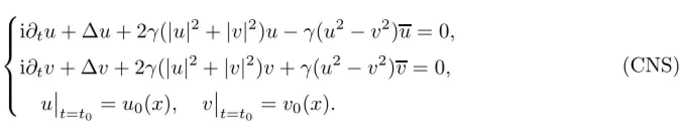
Note that the choice of the above parameters are not unique，it only needs to satisfy the conditionµ1=µ2＞γ＞0.

The purpose of this article is to study the Cauchy problem of（CNS），we obtain the global existence of L2and H1solution in n=1，2，3，and two sharp conditions for global existence and blow up in two and three space dimension are also obtained.We organize this article as follows. Section 2 is rather standard；local Cauchy problem is studied in L2and H1.In Section 3，we deduce the conservation laws and global solutions of（CNS）.Finally，two sharp conditions for global existence and blow up are proved in Section 4.

2　Local Cauchy Problem

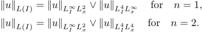
In this Section，we study local Cauchy problem for the system（CNS）.Now，we collect some basic notations and lemmas which will be used subsequent subsections.For any p with 1≤p≤∞，=Lp（Rn）denotes the Lebesgue space on Rn，and Wk，pdenotes the usual sobolev space of order k built on Lp.In particular，when p=2，Wk，pis also written Hk. For any interval I，we denote the Strichartz spaceas the space of strongly measurable function f from I to Lr（Rn）such thatFor 1≤p≤∞，p′is the dual exponent defined by=1，we denoteFor any a，b∈R，a∨b=max（a，b）.

For simplicity，we denoteRRnfdx byRRnf and various positive constants by C throughout this article.

The Cauchy problem for（CNS）with initial data（u（t0），v（t0））=（u0，v0）will be treated in the form of following system of integral equations

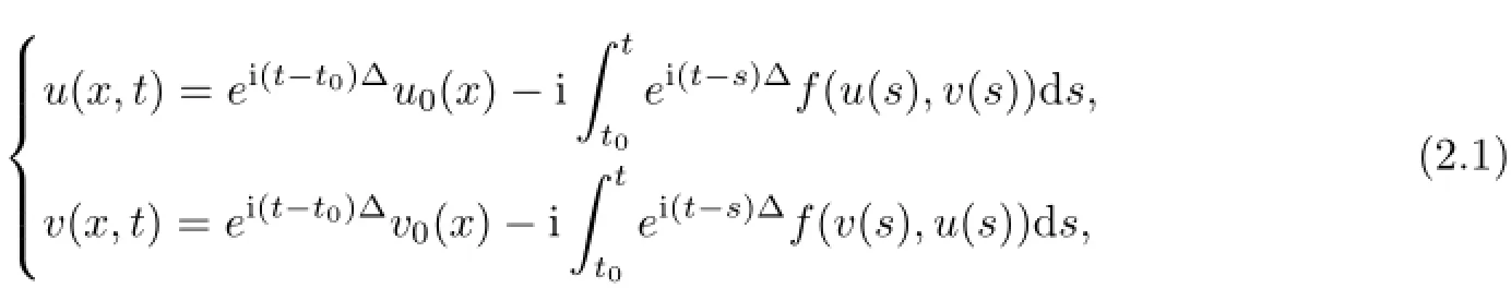
where f（u，v）=2γ（|u|2+|v|2）u−γ（u2−v2）u.

Next，let us recall the notion of admissible index-pairs.

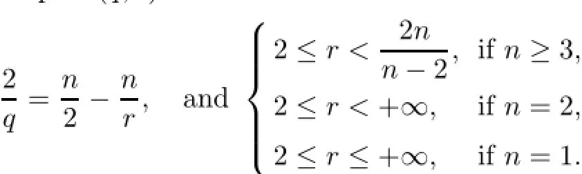
Definition 2.1The pair（q，r）is called admissible if

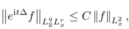
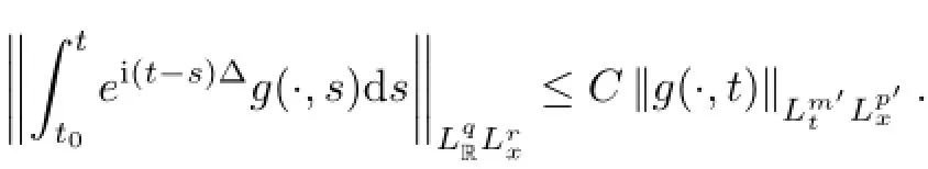
The well known Strichartz estimates for the Schrüodinger group S（t）=eit∆are recounted in the next lemma（see［3］for more details）.We will use the following estimates without particular comments.

Lemma 2.2If（q，r），（m，p）are admissible，then the group｛eit∆｝t∈Rsatisfies

and

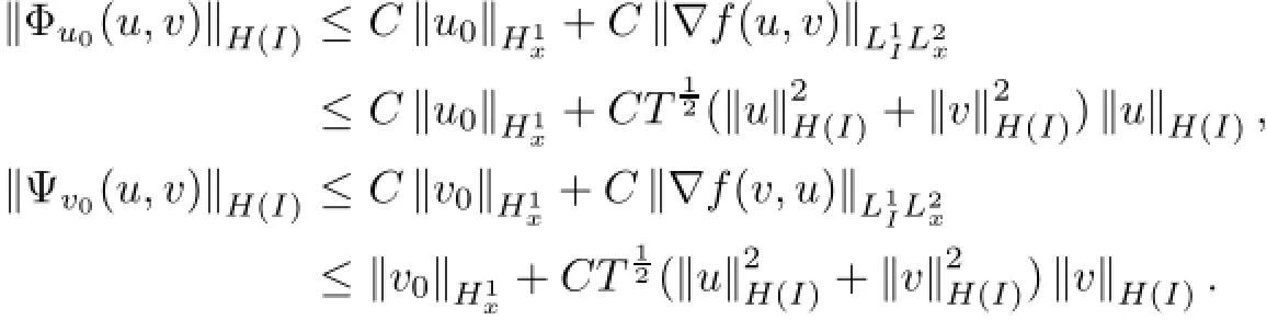
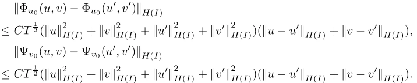
We use the above lemma to study the local Cauchy problem to（CNS）by a contraction argument.To be more specific，local solutions of（CNS）are constructed as a pair of fixed point（u，v）of contraction mapping（u，v）（Φu0（u，v），Ψv0（u，v）），where

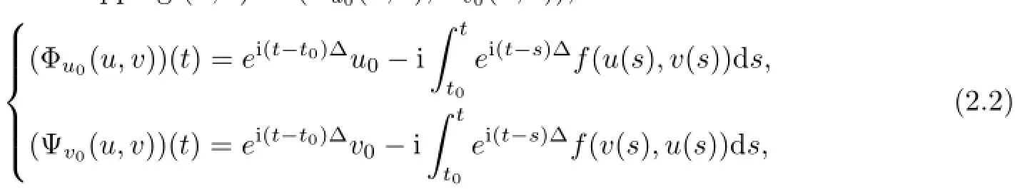
on a suitable complete metric space of functions on I：［t0−T，t0+T］for some T＞0 and f（u，v）=2γ（|u|2+|v|2）u−γ（u2−v2）u.

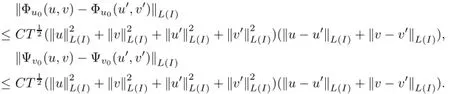
Remark 2.3For f（u，v）=2γ（|u|2+|v|2）u−γ（u2−v2）u，we have the following estimates：

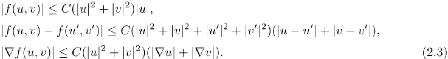
By（2.3），we have

2.1Local L2solution

By the standard scaling argument，it is natural to study（CNS）in L2for n≤2.For any u0，v0∈L2，we solve（CNS）in the following spaces：

on the interval I：［t0−T，t0+T］with T＞0.The corresponding norms are defined as follows：

We have the following local existence result.

Theorem 2.4If n=1，then for any a＞0 there exists T（a）＞0 such that for any（u0，v0）∈L2×L2with||u0||L2x∨||v0||L2x≤a，（CNS）has a unique pair of solutions（u，v）∈L（I）×L（I）with I=［t0−T（a），t0+T（a）］.If n=2，then for any（u0，v0）∈L2×L2，there exists T（u0，v0）＞0 such that（CNS）has a unique pair of solutions（u，v）∈L（I）×L（I）with I=［t0−T（u0，v0），t0+T（u0，v0）］.

ProofWe first consider the case n=1.We estimate Φu0（u，v）and Ψv0（u，v）as follows：

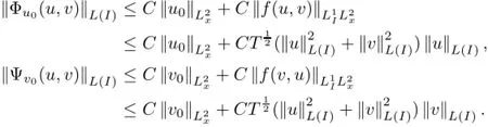
Similarly，we have

Then，the standard contraction argument on（u，v）→（Φu0（u，v），Ψv0（u，v））on a closed ball in L（I）×L（I）goes through by taking T＞0 sufficiently small with respect to a＞0 via radius of the ball.This yields the existence and uniqueness of local solutions on［t0−T，t0+T］under the size restriction on the radius.The uniqueness of solutions without the size restriction of the radius follows by a similar argument by taking the size of successive time interval sufficiently small.

Next，we consider the case n=2.We estimate Φu0（u，v）and Ψv0（u，v）as follows：

Similarly，we have

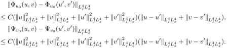
There exists δ＞0 such that if（u0，v0）∈L2×L2，we have

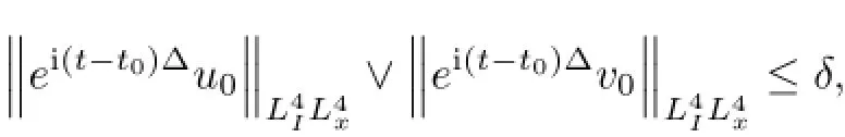
if we take T＞0 sufficiently small.We choose a closed ball B in Strichartz spacewith center at the origin and radius 2δ，such that（B，d）is a complete metric space withtherefore，we can complete the contraction argument.The solution satisfies the integral equations（2.2）and by Strichartz estimate the solution belongs to L（I）×L（I）.The proof of Theorem 2.4 is concluded.

2.2Local H1solution

By the standard scaling argument，it is natural to study（CNS）in H1space for n≤4. More precisely，for u0，v0∈H1，we solve（CNS）in the following spaces：

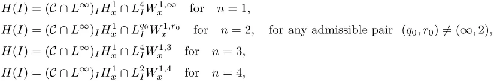
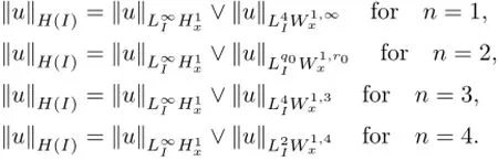
on the interval I：［t0−T，t0+T］with some T＞0.The corresponding norms are defined as follows：

We have the following local existence result.

Theorem 2.5If n≤3，then for any a＞0，there exists T（a）＞0 such that for any（u0，v0）∈H1×H1with||u0||H1∨||v0||H1≤a，then（CNS）has a unique pair of solutions（u，v）∈H（I）×H（I）with I=［t0−T（a），t0+T（a）］.If n=4，then for any（u0，v0）∈H1×H1，there exists T（u0，v0）＞0 such that（CNS）has a unique pair of solutions（u，v）∈H（I）×H（I）with I=［t0−T（u0，v0），t0+T（u0，v0）］.

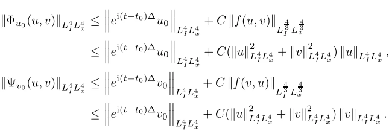
ProofWe first consider the case n=1.We estimate Φu0（u，v）and Ψv0（u，v）as follows：

Similarly，we have

From the above estimates，the conclusion follows for n=1.Next，considering n≥2，in this case the pairis admissible and the dual pair is given byBy Hüolder inequality

and Sobolev embedding，we have the following estimate

then the conclusion follows in a similar way as in the proof of Theorem 2.4.The proof of Theorem 2.5 is concluded.

3　Global Existence for n=1

3.1Global L2solution

Let n≤2 and（u，v）be the unique local solution given by Theorem 2.4，then we obtain

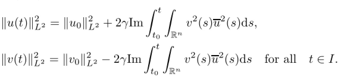
We have the following assertion concerning the conservation of total charge.

Proposition 3.1Let n≤2 and（u，v）be the unique local solution given by Theorem 2.4. Then，（u，v）satisfies the following conservation law：for any t∈I.

Remark 3.2In fact，the conservation of total charge is valid for all 1≤n≤4.Moreover，we see that the difference between the ICNLS（γ=0）and CCNLS（γ 6=0）is that in the ICNLS case，mass is conserved for each of the two components，whereas in the CCNLS case，only the total mass is conserved and component masses are not conserved.

We state the global L2solutions on the function space L（R），where

Theorem 3.3Let n=1，then for any（u0，v0）∈L2×L2，（CNS）has a unique pair of solutions（u，v）∈L（R）×L（R）.In addition，M（t）=M（t0）for any t∈R.

ProofThe conclusion follows from Theorem 2.4 and Proposition 3.1 by the standard continuation argument of local solution.

3.2Global H1solution

Let n≤4 and（u，v）be the unique local solution given by Theorem 2.5，then for all t∈I，we have

and

We have the following assertion concerning the conservation of total energy.

Proposition 3.4Let n≤4 and（u，v）be the unique local solution given by Theorem 2.5. Then，（u，v）satisfies the following conservation law：for all t∈I.

We give the global H1solutions on function space H（R）in one space dimension，where

Theorem 3.5Let n=1，then for any（u0，v0）∈H1×H1，（CNS）has a unique pair of solutions（u，v）∈H（R）×H（R）with initial value（u0，v0）.

ProofWe recall the Gagliardo-Nirenberg inequality（［15］）for 1≤n≤3：

By（3.3），conservation of charge，energy and Young's inequality，we could estimate the coupling term as follows：

We obtain a priori estimate and the conclusion follows from a standard continuation argument. The proof of Theorem 3.5 is concluded.

Let us consider the case n=2，in this case

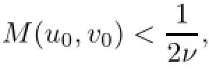
Theorem 3.6Let n=2.For any（u0，v0）∈H1×H1with

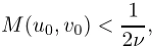
where ν is the best constant of Gagliardo-Nirenberg type inequality

then（CNS）has a unique pair of solutions（u，v）∈H（R）×H（R）with initial value（u0，v0）.

ProofWe have by the Gagliardo-Nirenberg inequality

This implies that

Therefore，the conservation of charge tells that if we choose initial data small，namely

then H1×H1seminorm will be uniformly bounded.A standard continuation argument establishes the global existence of the solution for（CNS）.

Remark 3.7We refer to［15］and［8］for related results concerning the proof for the existence of the ground state（Q，R）for the stationary system and the optimal constant ν.

4　Global Existence and Blow up for n=2，3

In this section，we consider the global existence and blow up of（CNS）for n=2，3.We first calculate a virial identity in a standard way like［5，11］and then consider the blow up of（CNS）（see Theorem 4.1）.Finally，we study two sharp conditions of global existence and blow up of（CNS）（see Theorems 4.3 and 4.5）.

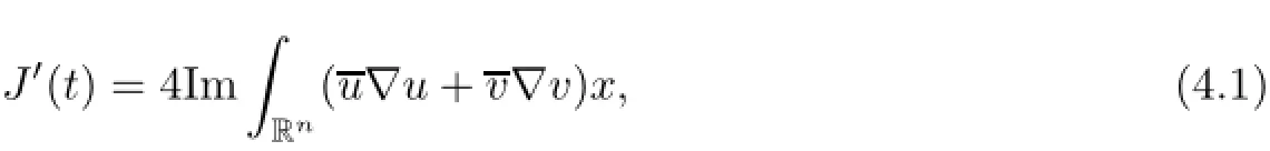
To be more specific，let ρ（x，t）∈C2（Rn+1）and set J（t）=RRnρ（t）（|u|2+|v|2）dx.After a regularization procedure，we have

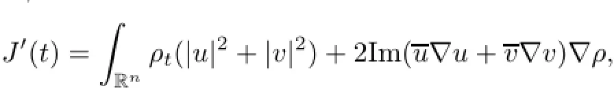
and

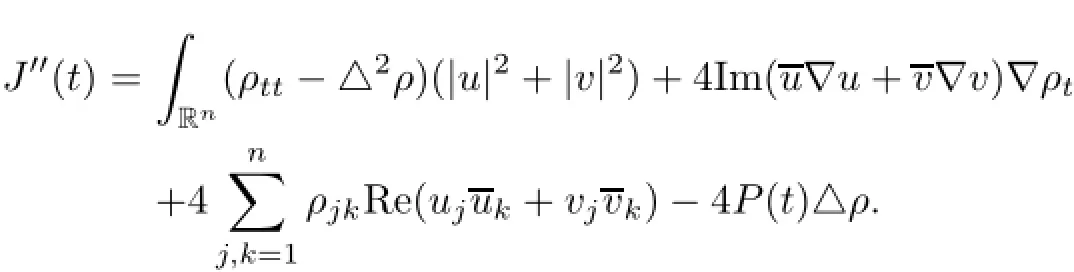
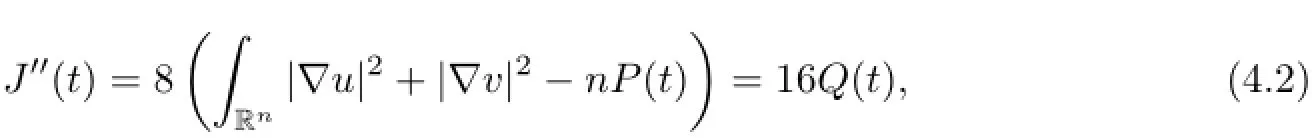
In particular，let ρ（x，t）=|x|2，then ρt=0，∇ρ=2x，ρjk=∂2jkρ=2δjk，so△ρ=2n，△2ρ=0. We obtain and where

We have the following assertion concerning finite-time blow up of（CNS）.

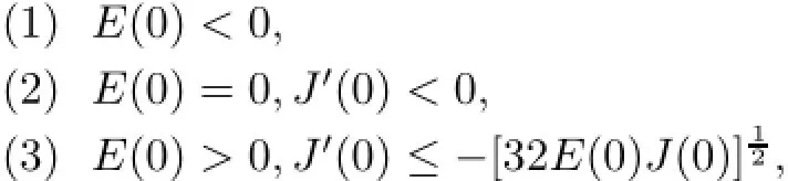
Theorem 4.1Let 2≤n≤3.Let（u0，v0）∈H1×H1satisfy（|x|u0，|x|v0）∈L2×L2and（u，v）be the corresponding pair of solutions given by Theorem 2.5 with t0=0.Then，the maximal existence time for（u，v）is finite in the following cases：

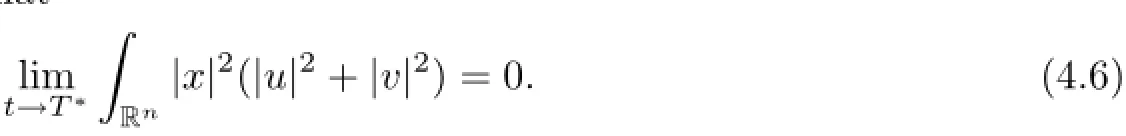
that is，there exists 0＜T∗＜+∞，such that

Before proving Theorem 4.1，we first give a lemma in［15］.

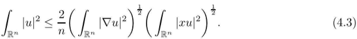
Lemma 4.2Let|x|u and∇u belong to L2.Then，we have u∈L2and the following inequality holds：

Proof of Theorem 4.1We argue by contradiction.Suppose the maximal existence time T of the solution is infinity.Then by assumption and（4.2），we obtain

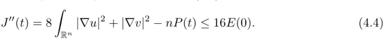
Integrating（4.4）with respect to t twice，one has

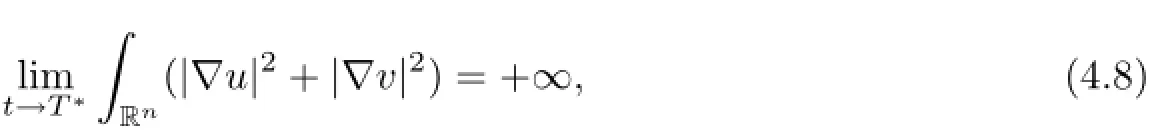
Under hypothesis（1），（2），or（3），（4.1）and（4.5），we deduce that if（u，v）∈H1×H1，then there exists some T∗∈R such that

By（4.3）and（3.1），we have

Letting t→T∗，one has

which implies that the maximal existence time T≤T∗＜+∞.The proof of Theorem 4.1 is concluded.

Next，we improve Theorem 4.1 to obtain two sharp conditions of global existence and blow up of（CNS）.

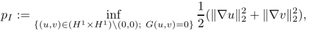
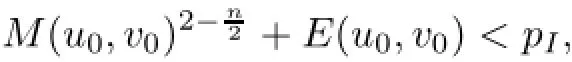
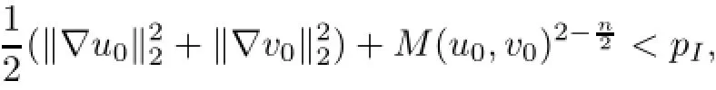
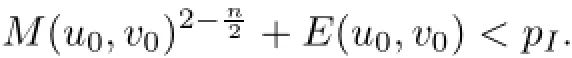
Theorem 4.3Assume that 2≤n≤3.The constrained variational problem where which satisfies pI＞0.Besides，if the initial data（u0，v0）∈H1×H1satisfies

then，we have the following assertions：

（1）If G（u0，v0）＞0，then the solution exists globally.

（2）If G（u0，v0）＜0，（|x|u0，|x|v0）∈L2×L2，then solution of（CNS）blows up in finite time.

Corollary 4.4Assume that 2≤n≤3.Then，if the initial data（u0，v0）∈H1×H1satisfies

the solution of（CNS）exists globally.

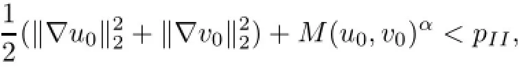
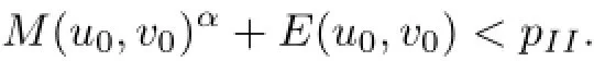
Theorem 4.5Assume that n=3，and let α＞0 be a fixed constant.The constrained variational problem

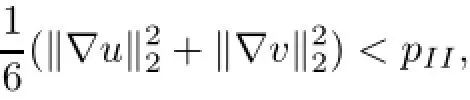
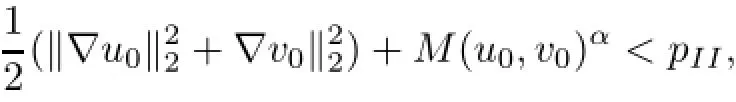
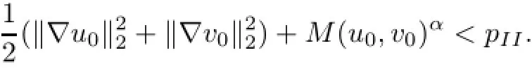
satisfies pII＞0.Besides，if the initial data（u0，v0）∈H1×H1satisfies

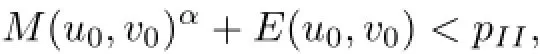
then we have the following assertions：

（1）If Q（u0，v0）＞0，the solution exists globally.

（2）If Q（u0，v0）＜0 and（|x|u0，|x|v0）∈L2×L2，the corresponding solution blows up in finite time.

Corollary 4.6Assume that n=3.If the initial data（u0，v0）∈H1×H1satisfies

then the solution of（CNS）exists globally.

We will follow the approach of［8，9，16］to prove the above theorems and corollaries.For reader's convenience，we first establish the invariant sets for（CNS）via three C0functionals M（u，v），E（u，v），and Q（u，v）.Our analysis can be formed as the following lemma.

Lemma 4.7Let F（u，v）and G（u，v）be two C0functionals on H1×H1.Let f（x，y）be a C0function on R2.Suppose that the cross-constrained minimization problem

satisfies p＞0.If in addition

then the sets

and

are all invariant sets of（CNS）on Rn.

ProofAssume that（u0，v0）∈W+，that is，G（u0，v0）＞0 and f（M（u0，v0），E（u0，v0））＜p. Noticing that M（u，v）and E（u，v）are conserved quantities of（CNS），we have

Next，we show that G（u，v）＞0.By contradiction，if G（u，v）≤0，then from the continuity，there exists a t1∈（0，T）such that G（u（t1），v（t1））=0 and（u（t1），v（t1））6=（0，0）.We infer from（4.9）that

which is a contradiction with the minimization of p.Thus，we obtain G（u，v）＞0 and

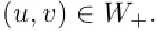
By the same argument，W−is also invariant under the flow generated by（CNS）.

Remark 4.8The idea of this proposition goes back to H.Berestycki and T.Cazenave［2］.［9］introduces the

to enlarge the invariant sets of the Schrüodinger equation on R2to the Schrüodinger system on Rnfor all n≥1.The power α＞0 in（4.10）relies on the Gagliardo-Nirenberg inequality.

We now state the strategy of the proof.Suppose we already get the fact that

andare invariant sets of（CNS）.Moreover，if we can show that there exist two constants M，δ such that

and

then we could draw the conclusion that（u0，v0）∈W+implies that the solution exists globally，and（u0，v0）∈W−implies that the solution blows up in finite time.In this sense，under the assumption f（M（u0，v0），E（u0，v0））＜p，we say G（u0，v0）=0 is a sharp condition between blow-up and global existence.

Next，we will prove Theorems 4.3，4.5 and Corollaries 4.4，4.6.

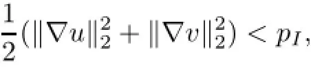
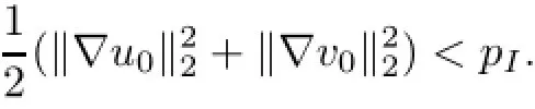
Proof of Theorem 4.3Step 1.We claim that the constrained variational problem in Theorem 4.3 satisfies pI＞0.For（u，v）∈H1×H1｛（0，0）｝subjected to G（u，v）=0，it follows from（3.3）that

which indicates that pI＞0.

Step 2.Choosing F（u，v）=12（‖∇u‖22+‖∇v‖22）and f（M，E）=M2−n2+E in Lemma 4.7，we see that

and

are invariant sets of（CNS）.

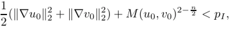
Step 3.Assume that（u0，v0）satisfies G（u0，v0）＞0.Then from Step 2，we have G（u，v）＞0 and M（u，v）2−n2+E（u，v）＜pI，which imply

and consequently the solution exists globally.

Step 4.Assume that（u0，v0）satisfies G（u0，v0）＜0.From Step 2，we have G（u，v）＜0 and M（u，v）2−n2+E（u，v）＜pI.

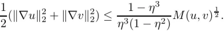
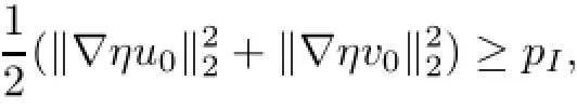
Case（1）n=2.In this case，Q（u，v）=E（u，v）=E（u0，v0）.From G（u0，v0）＜0，there exists an η∈（0，1）such that G（ηu0，ηv0）=0，that is，

Then，it follows from the minimization of pIthat

Inserting（4.11）into（4.12）yields

that is，

Thus，we have J′′（t）=16E（u0，v0）＜0 and the solution blows up in finite time.

Case（2）n=3.In this case，for any fixed t∈（0，T），there exists an η∈（0，1）such that G（ηu，ηv）=0，that is，

Then，it follows from the minimization of pIthat

Inserting（4.13）into（4.14）yields

that is，

On the other hand，

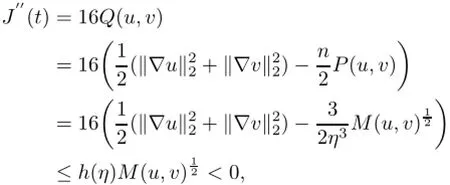
where

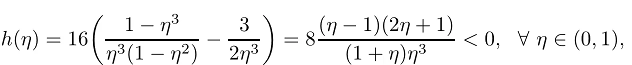
is used in the last step.Thus，we have J′′（t）＜0，and the solution blows up in finite time.The proof of Theorem 4.3 is concluded.

Proof of Corollary 4.4From the assumption

it is easy to see that

By Theorem 4.3，we only need to check that G（u0，v0）＞0.We argue by contradiction.If not，one would have G（u0，v0）≤0.Due to the minimization of pI，G（u0，v0）6=0.So，if G（u0，v0）＜0，then there exists an η∈（0，1）such that G（ηu0，ηv0）=0 and by the minimization of pI，we have

but which contradicts to the fact that

The proof of Corollary 4.4 is concluded.

Proof of Theorem 4.5Step 1.The constrained variational problem in Theorem 4.5 satisfies pII＞0.We argue by contradiction.Suppose there exists a sequence（uk，vk）∈（H1×H1）（0，0）satisfying Q（uk，vk）=0 and M（uk，vk）α+E（uk，vk）→0 as k→∞.By Q（uk，vk）=0，we get

which indicates that M（uk，vk）→0 and‖∇uk‖2→0 and‖∇vk‖2→0.On the other hand，by the Gagliardo-Nirenberg inequality，we get，from Q（uk，vk）=0，

that is，

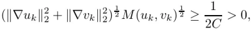
which contradicts to assumption M（uk，vk）→0，‖∇uk‖2→0，and‖∇vk‖2→0.

Step 2.Choosing F（u，v）=M（u，v）α+E（u，v）and f（M，E）=Mα+E in Lemma 4.7，we obtain the fact that

and

are invariant sets of（CNS）.

Step 3.Assume that u0，v0satisfies Q（u0，v0）＞0.Then from Step 2，we have

which implies

and therefore the solution exists globally.

Step 4.Assume that u0，v0satisfies Q（u0，v0）＜0.From Step 2，we have Q（u，v）＜0 and M（u，v）α+E（u，v）＜pII.We claim

and following which the solution blows up in finite time.

We prove the above claim.Indeed，if Q（u，v）＜0，then there exist an η∈（0，1）such that Q（ηu，ηv）=0 and M（ηu，ηv）α+E（ηu，ηv）≥pII.Moreover，Q（u，v）＜0 implies that P（u，v）＞0.Next，we do calculation to obtain

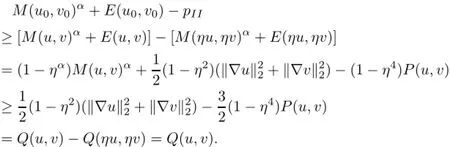
This concludes the proof of Theorem 4.5.

Proof of Corollary 4.6From the assumption

we see easily that

By Theorem 4.5，we only need to check that Q（u0，v0）＞0.We argue by contradiction；if not，one would have Q（u0，v0）≤0.Due to the minimization of pII，Q（u0，v0）6=0.So if Q（u0，v0）＜0，then there exists an η∈（0，1）such that Q（ηu0，ηv0）=0 and by the minimization of pII，we have

but which contradicts to the fact that

The proof of Corollary 4.6 is concluded.

References

［1］Agrawal G P.Nonlinear Fiber Optics.Optics and Photonics.Academic Press，2007

［2］Berestycki H，Cazenave T，et al.Instabilit´e des´etats stationnaires dans les´equations de Schrüodinger et de Klein-Gordon non lin´eaires.C R Acad Sci Paris，S´eire I，1981，293：489-492

［3］Cazenave T.Semilinear Schrüodinger Equations，Vol 10 of Courant Lecture Notes in Mathematics.New York：New York University，Courant Institute of Mathematical Sciences，2003

［4］Cazenave T，Weissler F B，et al.The Cauchy problem for the critical nonlinear Schrüodinger equation in Hs.Nonlin Anal，1990，14：807-836

［5］Glassey R T.On the blowing up of solutions to the Cauchy problem for nonlinear Schrüodinger equations. J Math Phys，1977，18：1794-1797

［6］Kanna T，Sakkaravarthi K，et al.Multicomponent coherently coupled and incoherently coupled solitons and their collisions.J Phys A：Math Theor，2011，44：285211

［7］Kivshar Y S，Agrawal G P，et al.Optical Solitons：From Fibers to Photonic Crystals.San Diego，CA，Academic Press，2003

［8］Li X G，Wu Y H，Lai S Y，et al.A sharp threshold of blow-up for coupled nonlinear Schrüodinger equations. Journal of Physics A：Mathematical and Theoretical，2010，43：165025

［9］Ma L，Zhao L，et al.Sharp thresholds of blow-up and global existence for the coupled nonlinear Schrüodinger system.J Math Phys，2008，49：062103

［10］Manakov S V.On the theory of two-dimensional stationary self-focusing of electromagnetic waves.Journal of Experimental and Theoretical Physics，1974，38：248-253

［11］Merle F.Determination of blow-up solutions with minimal mass for nonlinear Schrüodinger equations with critical power.Duke Math J，1993，69：427-454

［12］Ogawa T，Tsutsumi Y，et al.Blow-up of H1solution for the nonlinear Schrüodinger equation.J Diff Eq，1991，92：317-330

［13］Sakkaravarthi K，Kanna T，et al.Bright solitons in coherently coupled nonlinear Schrüodinger equations with alternate signs of nonlinearities.J Math Phys，2013，54：013701

［14］Sirakov B.Least energy solitary waves for a system of nonlinear Schrüodinger equations in RN.Comm Math Phys，2007，271：199-221

［15］Weinstein M I.Nonlinear Schrüodinger equations and sharp interpolation estimates.Comm Math Phys，1983，87：567-576

［16］Zhang J.Sharp threshold for blow-up and global existence in nonlinear Schrüodinger equations under a harmonic potential.Commun PDE，2005，30：1429-1443

December 11，2013；revised August 6，2015.This work is supported by the China National Natural Science Foundation under grant number 11171357.