S.Vahdati and D.Mirzaei

The Finite Points Approximation to the PDE Problems in Multi-Asset Options

S.Vahdati1and D.Mirzaei2

In this paper we present a meshless collocation method based on the moving least squares(MLS)approximation for numerical solution of the multiasset(d-dimensional)American option in financial mathematics.This problem is modeled by the Black-Scholes equation with moving boundary conditions.A penalty approach is applied to convert the original problem to one in a fixed domain.In finite parts,boundary conditions satisfy in associated(d−1)-dimensional Black-Scholes equations while in infinity they approach to zero.All equations are treated by the proposed meshless approximation method where the method of lines is employed for handling the time variable.Numerical examples for single-and two-asset options are illustrated.

Meshless methods,MLS approximation,finite points method,American options,Black-Scholes equation.

1 Introduction

Option is one of the interesting financial instruments which is the right(but not the obligation)to buy(call option)or sell(put option)a risky asset at a prescribed fixed price(exercise or strike price)on(European option)or before(American option)a given date called expiry date.Options are mostly modeled by partial or stochastic differential equations.The price of an American option is governed by a linear complementarity problem involving the Black-Scholes differential operator and a constraint(or obstacle)on the value of the option.For details see Huang and Pang(1998);Jaillet,Lamberton,and Lapeyre(1990);Wilmott,Dewynne,and Howison(1993).

To remove the free boundary conditions in an American option,a method whichadds a penalty term to the Black-Scholes equation can be employed.Using the penalty term is not quite new,for example,penalty method and front fixing method together with the finite difference method are discussed in Wu and Kwok(1997);Nielsen,Skavhaug,and Tveito(2002,2008);Pantazopoulos,Houstis,and Kortesis(1998).

There are several methods for numerical solution of European and American options.A lattice method,as the first numerical method to Black-Scholes equation proposed in Cax,Ross,and Rubinstein(1979).Finite difference methods(FDM)combined with PSOR algorithm(Yves and O.Pironneau(2005))and operator splitting method in(Dronen and Toivanen(2004))are other approaches.Space-time adaptive finite difference methods for European multi-asset options are proposed in Persson and Von Sydow(2007);Lötstedt,Persson,Von Sydow,and Tysk(2007).In spite of the method of Persson and Von Sydow(2007)which uses second-order formulas in combination with adaptivity,in Linde,Persson,and Von Sydow(2009)a high accurate adaptive finite difference solver is introduced for the Black-Scholes equation.However,due to the discontinuity of the first derivative of the final condition,these discretizations yield only second-order accuracy locally.To circumvent this problem,authors use an extra(fine)grid around the discontinuity in a limited space-and time-domain.In Persson and Von Sydow(2010)a numericalmethod for pricing American options,in two cases,constant volatility and stochastic volatility,is proposed which uses a space-time adaptive finite difference method.Lee and Kim(2012),proposed a local differential quadrature(LDQ)method to solve the option-pricing models with stochastic volatilities.

Finite volume methods are also used for pricing American/European option with constant or time-dependent volatility.For example Wang(2004);Wang,Yang,and Teo(2006)have proposed a fitted finite volume method for spatial discretization and an implicit time stepping technique for temporal discretization which is combined with power penalty method for option pricing.

Finite elementmethodsare more flexible formesh adaptivity.See Yvesand O.Pironneau(2005);Memon(2012);Young,Sun,and Shen(2009).In this scheme the analysis is performed within the framework of the vertical method of lines,where the spatial discretization is formulated as a Galerkin method with trial space spanned by proper basis functions like piecewise polynomials.

Recently,some papers have been published which consider the meshfree radial basis functions for solution of Black-Scholes equation for financial options.As examples see Fasshauer,Khaliq,and Voss(2004);Hon and Mao(1999);Hon(2002);Pettersson,Larsson,Marcusson,and Persson(2005).In Fasshauer,Khaliq,and Voss(2004)a penalty method is presented to handle the moving boundary in American options.This technique will be used in the present paper.It is known that RBF techniques suffer from the ill-conditioned interpolation matrix.The condition numbers are sometimes increased exponentially.To overcome this drawback some precautions like preconditioning should be applied.We refer the reader to Beatson,Cherrie,and Mouat(1999);Brown,Ling,Kansa,and Levesley(2005);Fornberg and Piret(2007);Fornberg,Larsson,and Flyer(2011);Fornberg,Lehto,and Powell(2013)for details.

Moving least squares(MLS)approximation is another class of meshfree approximation methods which has been widely used in numerical solutions of PDEs.Some applications can be found in Belytschko,Krongauz,Organ,Fleming,and Krysl(1996);Atluri and Zhu(1998);Atluri and Shen(2002);Atluri(2005);Sladek,Sladek,and Atluri(2004).MLS is a stable numerical approximation with polynomial order of accuracy.In contrast with the global RBFs,the final approximation matrix is often well-conditioned.In this paper,we use the MLS as trial approximation to build a collocation scheme for penalized Black-Scholes equation in option pricing.This method is usually called finite points method.No background mesh is required for numerical simulation because the method uses scattered points to represent the consideration domain.

It should be noted that Yongsik,Hyeong-Ohk,and Hyeng Keun(2014)applied a meshfree method based on diffuse approximation of derivatives to solve option pricing in the single-asset case for European,Asian and Double barrier options.The present paper is different from that of Yongsik,Hyeong-Ohk,and Hyeng Keun(2014)because it concerns multi-asset American options instead.Besides,the approximation method of this paper uses the standard derivatives of the MLS instead of diffuse derivatives.Diffuse derivatives can be obtained via a generalized moving least squares approximation as discussed in Mirzaei,Schaback,and Dehghan(2012)and can be easily applied to the problem of this paper,too.

The rest of paper is organized as below.In Section 2 the Black-Scholes model and the penalty approach are discussed.In Section 3 the MLS approximation is reviewed and in Section 4 the finite points method is developed for multi-asset American options.Finally,in Section 5 some numerical results are given.

2 American options and a penalty formulation

Following Fasshauer,Khaliq,and Voss(2004),assume that there are d assets whose prices at time t are denoted by S(t)=(S1(t),...,Sd(t)).We can determine the value of f(S,t)of the American put option by solving the d-dimensional Black-Scholes equation accompanying with moving boundary conditions.An American option problem is a free boundary problem because of the possibility of early exercise at any point during its life.For more details see Wilmott(1998);Brandimarte(2006).If the moving boundary is denoted by notation S(t)=(S1(t),...,Sd(t)),the time of expiry time by T,the volatility of i-th underlying asset by σi,the risk free interest rate by r,the dividend paid by asset i by Diand the correlation between assets i and j by ρij,then the following Black-Scholes equation with moving boundary conditions and payoff function(terminal condition)

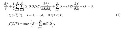
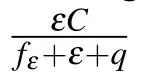
If we assume Ω={(S1,...,Sd):Si>0,i=1,...,d},by adding the penalty term to the original Black-Scholes equation we will have the following nonlinear PDE for S∈Ω and 0 6 t＜T,

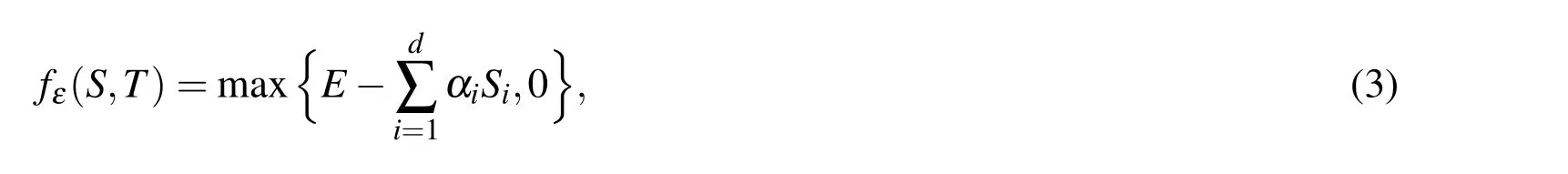
The terminal condition in time t=T is enforced by

and the boundary conditions are

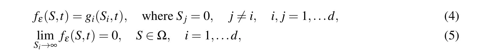
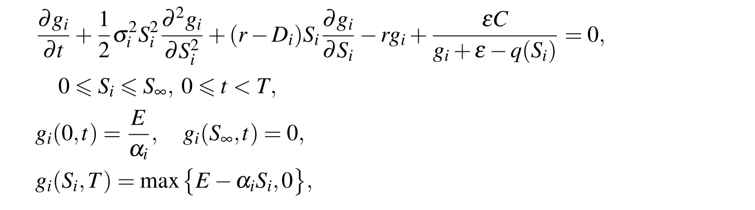
where q(Si)=E−αiSi.

3 MLS for trial approximtion

Meshlessormeshfree methodswrite everything entirely in termsof scattered points and this is an alternative to the mesh-based approximation methods like as finite element and finite volume methods.The radial basis functions(RBFs)are frequently used as meshless approximations in recent years.Another family of mostly used meshfree methods are moving least squares(MLS)and related methods,introduced by Lancaster and Salkauskas(1981).Applications of MLS for numerical solution of PDEs have come to the picture by diffuse element method(see Nyroles,Touzot,and Villon(1992)),element-free Galerkin method(see Belytschko,Lu,and Gu(1994)),meshless local Petrov-Galerkin(MLPG)methods(see Atluri and Shen(2002);Atluri and Zhu(1998);Dong,Alotaibi,Mohiuddine and Atluri(2014);Zhang,Dong,Alotaibi and Atluri(2013)),etc.

Here we aim to apply the MLS collocation method for the nonlinear equation(2)with the terminal and boundary conditions(3)-(5).But before that we explain the MLS approximation itself.Suppose that Ω is a closed subset of Rdand let

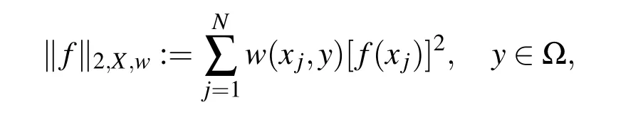
induced by the inner product

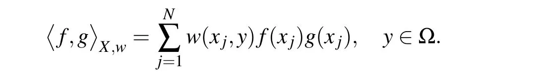
The inner product depends on moving point y∈Ω.This finally leads to a local approximation if y is chosen properly.If for x∈Ω we define

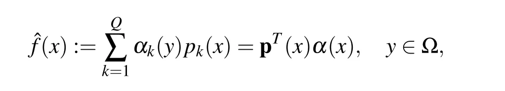
then from the theory ofbestapproximation in pre-Hilbertspaces,α(y)=(α1(y),...,αQ(y))Tshould be chosen such that

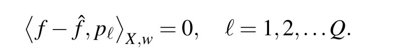
This leads to the normal system

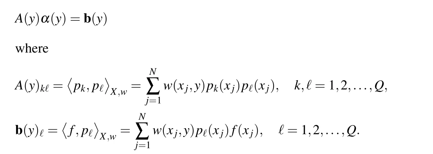
We noted that y should selected properly.In MLS to have a local approximation we put y:=x where x is current evaluation point,and the weight function w:Ω×Ω→R+∪{0}is defined such that it becomes smaller the further away its arguments are from each other.Ideally,w vanishes for arguments x,xj∈Ω with k x−xjk2greater than a certain threshold,say δ.Such a behavior can be modeled by using a translation-invariant weight function.This means that w is of the form

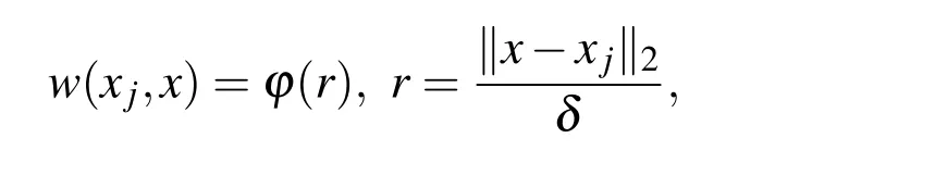
where δ is the scaling parameter and ϕ(r)＞ 0 for r∈ [0,1]and ϕ(r)=0 for r＞ 1.Let I(x)is the set of active indices in x,i.e.I(x)={j:k x−xjk 6 δ}and let Xx={xj,:j∈I(x)}.If we define

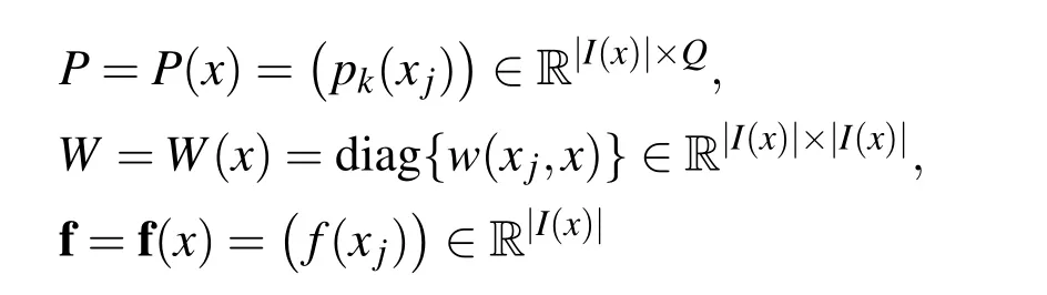
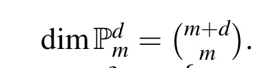
where|I(x)|denotes the size of I(x),then we clearly have A(x)=PTW P and b(x)=PTW f.According to Wendland(2005)if Xxis Pdm-unisolvent then A(x)is positive definite and the MLS approximation is well-defined at x.Solving the normal equation gives

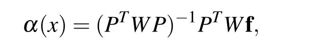
which leads to

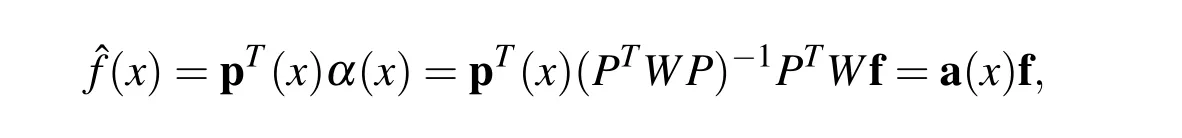
where a(x)=pT(x)(PTW P)−1PTW is called shape function vector at x.The extended form of the above equation can be written as

The MLS approximation is known to be a stable numerical algorithm,because as it was proven in Wendland(2005)

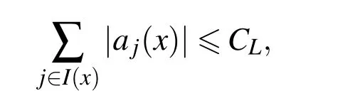
where CLis a small constant independent of X.This means that the Lebesgue functions are uniformly bounded by CL.The reader should compare this with the known results on polynomial interpolation.MLS is computationally attractive because it solves for every point x a locally weighted least squares problem which is turn out to be a very efficient method because it is not necessary to set up and solve a large system of equations.

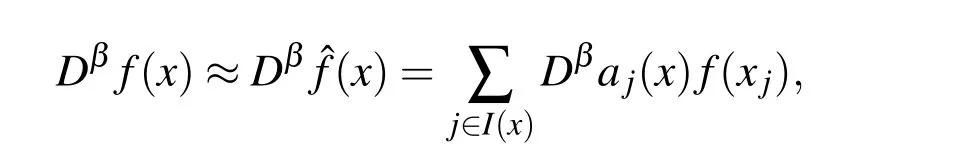
where β is a multi-index.It remains to show that how derivatives of ajcan be calculated.More details may be found in MLS literatures and specially in Belytschko,Krongauz,Organ,Fleming,and Krysl(1996).

Here we use the C0Gaussian weight function

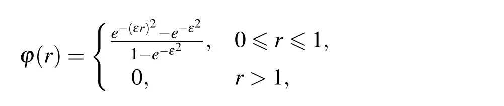
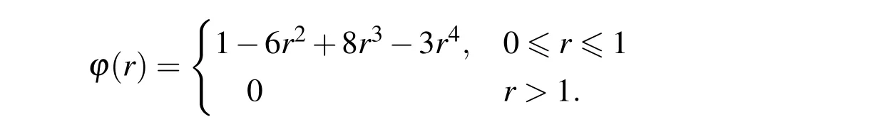
where ε is a shape parameter,and/or the C2spline weight function

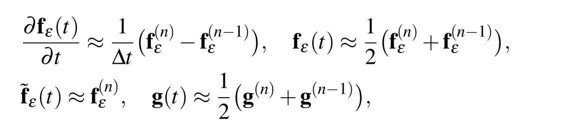
4 Numerical algorithm

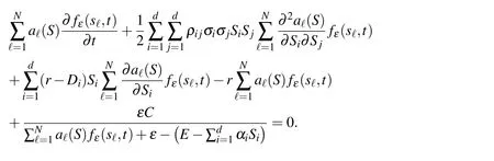
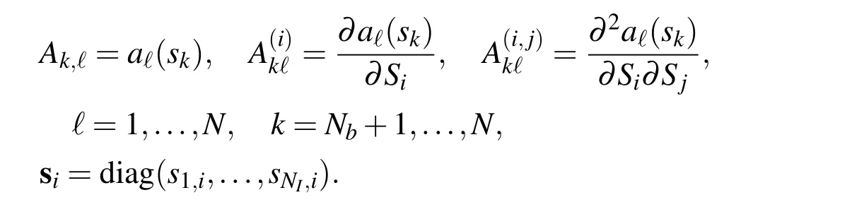
If we apply the above equation at internal test points S=sk,k=1,...,NI,in a vector form we have

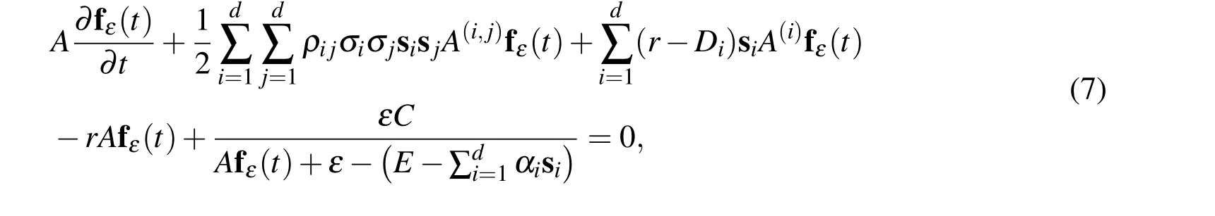
where we introduced the following notations

In a short notation,equation(7)can be rewritten as

Note that,in the above formulation,constants C,ε and E are interpreted as constant vectors of size NI,and the division and multiplication in the third term are elementby-element operators.

The terminal condition(3)provides the primary vector solution at t=T,i.e.

To enforce the boundary conditions,we should solve some one dimensional problems(d=1).In this case fε(0,t)=E and fε(S∞,t)=0.If MLS is applied,we have

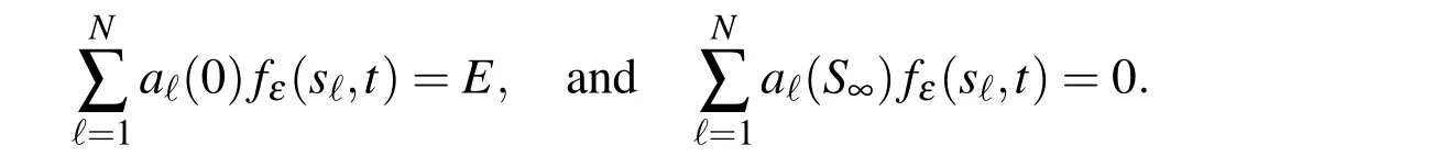
In vector form,

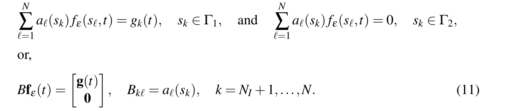
Equations(8)-(10)form a system of Differential Algebraic Equations(DAE).For a d-dimensional problem,due to(4),the corresponding(d−1)-dimensional problem should be solved to provide the values at half part of the boundary,say Γ1.The boundary conditions at the remaining parts(say Γ2)are zero due to(5).Thus the subroutines of lower dimensional problems should be called,inductively.Let g(t)be the vectorsolution ofcorresponding(d−1)-dimensionalproblem overboundary Γ1.Then

5 Numerical results

Here some numerical experiments are given for single and multi-asset options.To compare the results with the results of finite difference and RBF interpolation methods of Fasshauer,Khaliq,and Voss(2004)we consider only the case ε=0.01.The effect of this penalty parameter are extensively studied in Nielsen,Skavhaug,and Tveito(2008,2002).The Gaussian and spline weight functions for MLS approximation and different values for degree of polynomial basis functions(m)are considered.In all cases regular node distributions with mesh-sizehare used,although the method can always work for scattered data.The size supportδof weight functionwshould be large enough to ensure the regularity of matrixA(x)in MLS approximation.Indeedδshould depend on the density of nodes and the degree of polynomial basis functions.Hereδ=2mhis used.The shape parameterεin Gaussian weight function effects the numerical results,and unfortunately there is no optimal value available for that.Experiments show thatm6ε6 3mproduce accurate results.Hereε=2mis used.

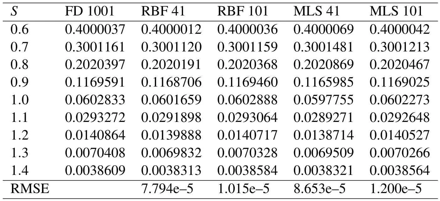
Table 1:Comparing finite difference,RBF and finite points solutions

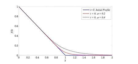
Figure 1:Initial(t=T=1),and final(t=0)profiles for two values of σ.

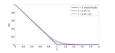
Figure 2:Initial(t=T=1),and final(t=0)profiles for two values of D.

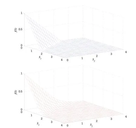
Figure 3:Initial(t=T=1),and final(t=0)profiles for correlated(ρ12=0.5)case.

For the single-asset option we setr=0.1,σ=0.2,D=0,E=1,T=1,S0=0,S∞=2 and use the Crank-Nicolson scheme in time with ∆t=0.01.Results are presented in the last two columns of Table 1 and compared with the finite difference(with many points as a reference solution)and the radial basis function(RBF)solutions of Fasshauer,Khaliq,and Voss(2004).Numbers in the first row of Table 1 represent the number of points used in numerical simulation for each method.

For a two-asset problem we user=0.1,σ1=0.2,σ2=0.3,α1=0.6,α2=0.4,D1=0.05,D2=0.01,E=1,T=1 and bΩ=[0,4]×[0,4].The time difference method withθ=0.5 is again employed.In Figure 3 the terminal profile and the profile att=0 are plotted in the case of correlated assets(σ12=0.5).Results are in excellent agreement with those given in Fasshauer,Khaliq,and Voss(2004).

In Figure 1 the profiles att=0 are plotted for different values ofσ.Other parameters remain unchanged.In Figure 2 the profiles forD=0 andD=0.1 are compared.

Atluri,S.;Zhu,T.-L.(1998): A new meshless local Petrov-Galerkin(MLPG)approach in computational mechanics.Computational Mechanics,vol.22,pp.117–127.

Atluri,S.N.(2005):The meshless method(MLPG)for domain and BIE discretizations.Tech Science Press,Encino,CA.

Atluri,S.N.;Shen,S.(2002):The Meshless Local Petrov-Galerkin(MLPG)Method.Tech Science Press,Encino,CA.

Beatson,R.K.;Cherrie,J.B.;Mouat,C.T.(1999): Fast fitting of radial basis functions:Methods based on preconditioned GMRES iteration.Advances in Compuational Mathematics,vol.11,pp.253–270.

Belytschko,T.;Krongauz,Y.;Organ,D.;Fleming,M.;Krysl,P.(1996):Meshlessmethods:an overview and recentdevelopments.ComputerMethodsinApplied Mechanics and Engineering,special issue,vol.139,pp.3–47.

Belytschko,T.;Lu,Y.;Gu,L.(1994):Element-Free Galerkin methods.International Journal for Numerical Methods in Engineering,vol.37,pp.229–256.

Brandimarte,P.(2006):Numerical Methods in Finance and Economics,A MATLAB-Based Introduction.2nd edition.Wiley.

Brown,D.;Ling,L.;Kansa,E.J.;Levesley,J.(2005):On approximate cardinal preconditioning methods for solving PDEs with radial basis functions.Engineering Analysis with Boundary Elements,vol.19,pp.343–353.

Cax,J.C.;Ross,S.A.;Rubinstein,M.(1979): Option pricing:a simplified approach.Journal of Financial Economics,vol.7,pp.229–263.

Dong,L.;Alotaibi,A.;Mohiuddine,S.A.;Atluri,S.N.(2014):Computational methods in engineering:a variety of primal&mixed methods,with global&local interpolations,for well-posed or ill-posed BCs.CMES:Computer Modeling in Engineering&Sciences,vol.99,no.1,pp.1–85.

Dronen,S.;Toivanen,J.(2004):Toivanen,operator splitting methods for American option pricing.Applied Mathematics Letters,vol.11,pp.809–814.

Fasshauer,G.E.;Khaliq,A.Q.M.;Voss,D.A.(2004): Using meshfree approximation for multi-asset American option problems.Journal of the Chinese Institute of Engineers,vol.27,pp.563–571.

Fornberg,B.;Larsson,E.;Flyer,N.(2011):Stable computations with gaussian radial basis functions.SIAM Journal on Scientific Computing,vol.33,pp.869–892.

Fornberg,B.;Lehto,E.E.;Powell,C.(2013): Stable calculation of gaussianbased rbf-fd stencils.Computers&Mathematics with Applications,vol.65,pp.627–637.

Fornberg,B.;Piret,C.(2007): A stable algorithm for at radial basis functions on a sphere.SIAM Journal on Scientific Computing,vol.30,pp.60–80.

Hon,Y.C.(2002): A quasi-radial basis functions method for American options pricing.Computer Mathematics with Applications,vol.43,pp.513–524.

Hon,Y.C.;Mao,X.Z.(1999):A radial basis function method for solving options pricing model.Financial Engineering,vol.8,pp.31–49.

Huang,J.;Pang,S.(1998):Option pricing and linear complementarity.Journal of Computational Finance,vol.2,pp.31–60.

Jaillet,P.;Lamberton,D.;Lapeyre,B.(1990): Variational inequalities and the pricing of American options.Acta Applicandae Mathematicae,vol.21,pp.263–289.

Lancaster,P.;Salkauskas,K.(1981): Surfaces generated by moving least squares methods.Mathematics of Computation,vol.37,pp.141–158.

Lee,J.E.;Kim,S.J.(2012): Simulation of multi-option pricing on distributed computing.CMES:Computer Modeling in Engineering&Sciences,vol.86,pp.93–112.

Linde,G.;Persson,J.;Von Sydow,L.(2009): A highly accurate adaptive finite difference solver for the black-scholes equation.International Journal of Computer Mathematics,vol.86,pp.2104–2121.

Lötstedt,P.;Persson,J.;Von Sydow,L.;Tysk,J.(2007):Space-time adaptive finite difference method for european multi-asset options.Computers and Mathematics with Applications,vol.53,pp.1159–1180.

Memon,S.(2012):Finite element method for American option pricing:a penalty approach.International Journal of Numerical Analysis and Modeling,Series B,vol.3,no.3,pp.345–370.

Mirzaei,D.;Schaback,R.;Dehghan,M.(2012):On generalized moving least squares and diffuse derivatives.IMA Journal of Numerical Analysis,vol.32,pp.983–1000.

Nielsen,B.F.;Skavhaug,O.;Tveito,A.(2002):Penalty and front-fixing methods for the numerical solution of American option problems.Journal of Computational Finance,vol.5,pp.69–97.

Nielsen,B.F.;Skavhaug,O.;Tveito,A.(2008):Penalty methods for the numerical solution of American multi-asset option problems.Journal of Computational and Applied Mathematics,vol.222,pp.3–16.

Nyroles,B.;Touzot,G.;Villon,P.(1992): Generalizing the finite element method:Diffuse approximation and diffuse elements.Computational Mechanics,vol.10,pp.307–318.

Pantazopoulos,K.N.;Houstis,E.N.;Kortesis,S.(1998): Front-tracking f inite difference methods for the valuation of American options.Computational Economics,pp.255–273.

Persson,J.;Von Sydow,L.(2007):Pricing european multi-asset options using a space-time adaptive fd-method.Computing and Visualization in Science,vol.10,pp.173–183.

Persson,J.;Von Sydow,L.(2010):Pricing american options using a space-time adaptive finite difference method.Mathematics and Computers in Simulation,vol.80,pp.1922–1935.

Pettersson,U.;Larsson,E.;Marcusson,G.;Persson,J.(2005):Option pricing using radial basis functions.In Leitao,V.;Alves,C.;Duarte,C.(Eds):ECCOMAS Thematic Conference on Meshless Methods.

Sladek,J.;Sladek,V.;Atluri,S.(2004):Meshless local Petrov-Galerkin method for heat conduction problem in an anisotropic medium.CMES:Computer Modeling in Engineering&Sciences,vol.6,pp.309–318.

Wang,S.(2004):A novel fitted finite-volume method for the black-scholes equation governing option pricing.IMA Journel of Numerical Analysis,vol.24,pp.699–720.

Wang,S.;Yang,X.Q.;Teo,K.L.(2006): Power penalty method for a linear complementarity problem arising from american option valuation.Journal of Optimization Theory and Applications,vol.129,pp.227–254.

Wendland,H.(2005):Scattered Data Approximation.Cambridge University Press.

Wilmott,P.(1998):Derivatives,The Theory and Practice of Financial Engineering.Wiley,New York.

Wilmott,P.;Dewynne,J.;Howison,S.(1993):Option pricing:Mathematical models and computation.Oxford Financial Press.

Wu,L.;Kwok,Y.(1997):A front-fixing finite difference method for the valuation of American options.Journal of Financial Engineering,pp.83–97.

Yongsik,K.;Hyeong-Ohk,B.;Hyeng Keun,K.(2014): Option pricing and greeks via a moving least square meshfree method.Quantitative Finance,vol.14,pp.1753–1764.

Young,D.L.;Sun,C.P.;Shen,L.H.(2009): Pricing options with stochastic volatilities by the local differential quadrature method.CMES:Computer Modeling in Engineering&Sciences,vol.86,pp.129–150.

Yves,A.;O.Pironneau,O.(2005):Computational methods for option pricing,vol.30 ofFrontiers in Applied Mathematics.SIAM,Philadelphia,PA.

Zhang,T.;Dong,L.;Alotaibi,A.;Atluri,S.N.(2013): Application of the MLPG mixed collocation method for solving inverse problems of linear isotropic/anisotropic elasticity with simply/multiply-connected domains.CMES:Computer Modeling in Engineering&Sciences,vol.94(1),pp.1–28.

1Department of Mathematics,Faculty of Mathematics and Computer Science(Khansar),University of Isfahan,81746-73441 Isfahan,Iran.E-mail:s.vahdati@khn.ui.ac.ir

2Department of Mathematics,University of Isfahan,81746-73441 Isfahan,Iran. E-mail:d.mirzaei@sci.ui.ac.ir