MA Hao （马皓）， QIU Xiang （邱翔）， LUO Jian-ping （罗剑平）， GU Pin-qiang （顾品强），LIU Yu-lu （刘宇陆）

1. School of Mechanical Engineering， Shanghai Institute of Technology， Shanghai 201418， China，E-mail： tracy_mahao@sina.com

2. School of Science， Shanghai Institute of Technology， Shanghai 201418， China

3. Shanghai Meteorological Service in Fengxian District， Shanghai 201416， China

4. Shanghai Institute of Applied Mathematics and Mechanics， Shanghai University， Shanghai 200072， China

Analysis of temperature time series based on Hilbert-Huang Transform*

MA Hao （马皓）1， QIU Xiang （邱翔）2， LUO Jian-ping （罗剑平）1， GU Pin-qiang （顾品强）3，LIU Yu-lu （刘宇陆）4

1. School of Mechanical Engineering， Shanghai Institute of Technology， Shanghai 201418， China，E-mail： tracy_mahao@sina.com

2. School of Science， Shanghai Institute of Technology， Shanghai 201418， China

3. Shanghai Meteorological Service in Fengxian District， Shanghai 201416， China

4. Shanghai Institute of Applied Mathematics and Mechanics， Shanghai University， Shanghai 200072， China

In this paper， with consideration of the nonlinear and non-stationary properties of the temperature time series， we employ the Hilbert-Huang Transform， based on the empirical mode decomposition （EMD）， to analyze the temperature time series from 1959 to 2012 in the Fengxian district of Shanghai， obtained from a certain monitoring station. The oscillating mode is drawn from the data，and its characteristics of the time series are investigated. The results show that the intrinsic modes of 1， 2 and 6 represent the periodic properties of 1 year， 2.5 years， and 27 years. The mean temperature shows periodic variations， but the main trend of this fluctuation is the rising of the temperature in the recent 50 years. The analysis of the reconstructed modes with the wave pattern shows that the variations are quite large from 1963 to 1964， from 1977 to 1982 and from 2003 to 2006， which indicates that the temperature rises and falls dramatically in these periods. The volatility from 1993 to 1994 is far more dramatic than in other periods. And the volatility is the most remarkable in recent 50 years. The log-linear plots of the mean time scales T and M show that each mode associated with a time scale almost twice as large as the time scale of the preceding mode. The Hilbert spectrum shows that the energy is concentrated in the range of low frequency from 0.05 to 0.1 Hz， and a very small amount of energy is distributed in the range of higher frequency over 0.1 Hz. In conclusion， the HHT is better than other traditional signal analysis methods in processing the nonlinear signals to obtain the periodic variation and volatility's properties of different time scales.

atmospheric turbulence， temperature time series， empirical mode decomposition （EMD）， Hilbert Huang Transform

Introduction

Global warming is currently attracting more and more attentions of researchers， and its causes and the effects on the global climate are issues under debate. In this context， the temperatures vary in different areas of the world. The global mean temperature has raised from 0.56oC to 0.92oC in recent 100 years［1］. The various climate factors in China， especially the average temperature， see complicated fluctuations. Zhao et al.［2］revealed that the climate warmingin China reaches 0.2oC-0.8oC in recent 100 years， Tang et al.［3］found the annual average temperaturein the surface in China has raised about 0.79oC since 1905， so the volatility of thelocaltemperature change is one of the core/key problems in the study of climate problems［4］. The volatility of the temperature variation is useful in identifying and evaluating the causes of the global warming， and it provides an essentialbasis to forecast the trend of the global warming［5］.

The Fengxian district is located in the south of Shanghai， to the north side of the Hangzhou Bay. Agriculture is the mainstay of its economy， in the planning of the Shanghai government. Therefore， the temperature change in this district is important for better understanding and analyzing the climate changes of the natural ecological environment. Due to its special geographic position， the climate in Fengxian isless influenced by the urban heat island than that in other highly urbanized areas in Shanghai. Comparing the annual mean temperature in Xujiahui with that in Fengxian， the difference between them was 0.1oC in 1960， 0.9oC in 1990， and 1.3oC in 2000. And the difference is becoming more and more important.Itis shownthat the temperature in Fengxian is in a rising trend since 1960［6］. From the beginning of the 21st century， under the background of the global warming，the intensity and the frequency of the extreme temperature have increased obviously. And the fluctuation of the temperature change in Fengxian is also more significant［7］.

In the study of the temperature time series， the multi-scaling structures of the oscillation were not paid enough attention. So we take up the multi-scaling structures based on the empirical mode decomposition（EMD） method introduced by Huang et al. as a new time series analysis technique， to separate a given time series into a sum of modes， each associated with well defined scales［8］. This method is very efficient for non-stationary and nonlinear time series， and in separating trends from small-scale fluctuations［9］. Due to its ability of characterizing the multiscaling scale invariant directly， the EMD method has met with a great success and has been successfully applied to many fields of natural and applied sciences： the water wave analysis［10］， the earthquake wave analysis， the meteorology and climate studies［8］， and the biological applications［11］， among others. It has already been applied to non-stationary temperature data， but most studies focus on the relationship between the time and the amplitude， not so much on the frequency. In this paper，we use the Hilbert spectral analysis to describe the relationship among the time， the amplitude and the frequency［12］.

The EMD is used to analyze the oscillating characteristics of the monthly mean temperature time series in the Fengxian district based on the modes after decomposing， the reconstructed modes with the wave pattern are used to analyze the oscillation characteristics of different time scales， the log-linear plot is used to show the relationship between the modes and the mean time scale， the Hilbert spectrum and the Hilbert marginal spectrum are used to reveal the relationship among the time， the frequency and the energy.

1. Empirical mode decomposition and Hilbert spectral analysis

1.1Data collection and preprocessing

The meteorological data， analyzed in this paper，is collected from the Shanghai meteorological service in the Fengxian district. The data include the monthly mean temperatures from 1959 to 2012， which can represent the temperature variation in the past 50 years in the Fengxian district. The monthly mean data are obtained from the averages of daily 2， 8， 14， 20 o'clock data， then with the consideration of the days in a month the arithmetic mean is taken， and the monthly average temperatures （1959-2012） recorded by the Fengxian observatory， Shanghai are analyzed here，including 648 months.

1.2Hilbert-Huang transform

The starting point of the EMD is that most of the signals are multi-components， which means that different scales exist simultaneously. The signal can be considered as a superposition of fast and slow oscillations at a very local level. In the time series analysis， a characteristic scale generally is explicitly or implicitly considered［13，14］. For example， in the Fourier analysis the characteristic scale is the length of one period of the sine （or cosine） wave. Then an integration operator is applied to extract the component information. The Fourier analysis is thus an energy based method［15］：only when a component contains enough energy， it can be detected by such method. The characteristic scale for the present EMD approach is defined as the distance between two successive maxima （or minima）points. This scale based definition gives the EMD a very local ability. According to the above definition of a characteristic scale， the so-called intrinsic mode function （IMF） is then proposed to approximate the mono-component signal， which satisfies the following two conditions［14，16］： （1） the difference between the number of local extrema and the number of zero-crossings must be zero or one， （2） the running mean value of the envelope defined by the local maxima and by the local minima is zero.

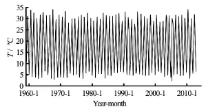
Fig.1 Original signal （1959-01-2012-12）

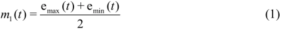
The EMD algorithm is proposed to extract the IMF modes from a given time series［14］. The first step of the EMD algorithm is to identify all local maxima（respectively， minima） points for a given time series x（t）. Once all local maxima points are identified， the upper envelopeemax（t）（respectively， the lower envelope emin（t）） is constructed by a cubic spline interpolation. The mean between these two envelopes is defined as：

Fig.2 The EMD decomposition of Fengxian monthly average temperature time series （1959-01-2012-12）

The first component is estimated by

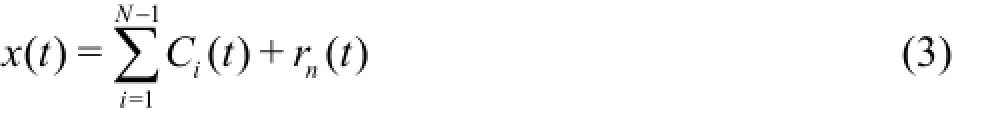
Ideally，h1（t）should be an IMF as expected. In reality， however，h1（t）may not satisfy the condition to be an IMF. We take h1（t）as a new time series and repeat the shifting processj times， until h1j（t）is an IMF. We thus have the first IMF componentC1t= h1j（t ）and the residual from x（t ）. The shifting procedure is then repeated on the residuals until rn（t）becomes a monotonic function or at most has one local extreme point. This means that no more IMF can be extracted fromrn（t）. Thus， with this algorithm we finally haven-1IMF modes with one residual rn（t）. The originalx（t ）is then rewritten as

A stopping criterion has to be introduced in the EMD algorithm to stop the shifting process.

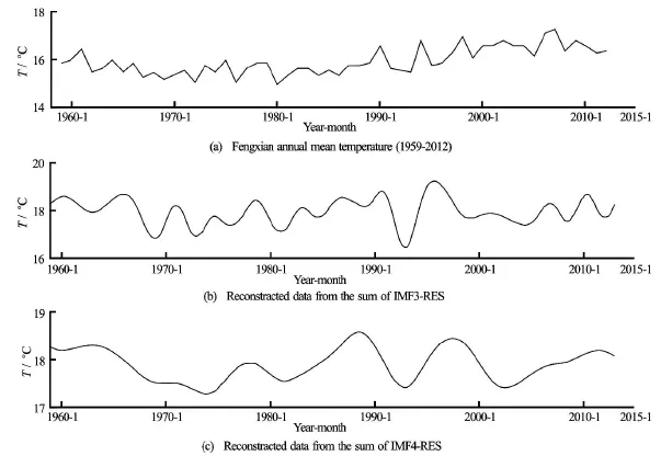
Fig.3 Comparison of reconstruction of the data from the IMFs with annual mean temperature

2. Monthly average temperature time series analysis

2.1EMD decomposition and the analysis of average temperature time series in Fengxian

The results over the entire data （see Fig.1）， are obtained after the EMD decomposing. Then 6 IMFs and a residual are obtained （see Fig.2）. From this figure， it is seen that there is a gradual increase of the time scale with the mode and each mode has a different mean frequency， from high frequency to low frequency.

In processing the non-linear temperature time series with the EMD method， the time series could be decomposed into IMFs of several time scales. The IMFs show some features， which can not be seen from the original series.

The IMF1 shows the high frequency oscillation，which well depicts Fengxian's temperature fluctuations in about 12 months. And it is plausible that the original time series volatility can be found in the IMF 1. Therefore， the IMF 1 can well reflect the fluctuation details of the monthly mean temperature time series in Fengxian. The IMF 2 shows the higher fluctuation in the average time scale. Besides， it is found that the fluctuationrange is enhanced from 1991 to 1998 than in other time scales. The IMF 6 reflects the change of the trend. From the observed residual， the temperature trend continuallyrises since the 1980s in Fengxian. Jiang［17］revealed that there are three temperature sharp risings， one of them is from the 1980s to the 1990s. Mu et al.［18］also found that the temperature of Shanghai suddenly starts to rise since 1979. In this paper， a similar result is found. Besides， a similar time point of the temperature change as in Fengxian is also found in Shanghai.

2.2Periodic analysis

Figure 2 shows that each mode has its frequency of fluctuation and a unique periodicity. Through reconstructing IMFs from 3 to the residual and from 4 to the residual （as Fig.3）， it is shown that their trends and periodicity are similar to those of the annual mean temperature time series in Fengxian.

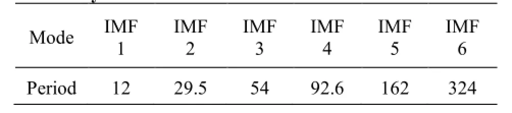
Table 1 Cycle of the IMFs

Through the above analyses， it is seen with the EMD method， that we can catch different periodic features from each mode （as shown in Table 1）. The properties of different time scales of non-linear temperature time series are essential for forecasting the temperature or preventing the disaster.

The relationship between the modem and the mean time scaleT is shown in Fig.4. The straight line in the log-linear plot suggests the following relationbetween the mean time scale Tandm ， for all modes

where T0=7.231is a constant and the coefficient λ=0.632is graphically estimated. Calculation shows thateλ=1.9is close to 2， which indicates that each mode is linked with a time scale almost twice as large as the time scale of the preceding mode， which is consistent to a dyadic filter bank in the time domain. It is a good analysis method for periodic changes in nonlinear time series.

Fig.4 Mean time scales associated with each mode

2.3Analysis of variability

With the EMD method， the behaviour of different frequencies can be acquired. But one has to consider different temperatures in different times. To further study different temperatures， therefore， we take up the variability， to measure the fluctuation ratio between each mode and the original data.

Fig.5 The volatility （a） and variability （b） of reconstructed data from the sum of IMF 2-IMF 6

We define the variability as the ratio between the absolute value of the IMF in any time and the original data. The variability is expressed as［19］

where Sh（t ）is defined as

The main period change in IMF 1 is obtained，and the special signal intensity and its period change can be obtained in IMF 1. Figure 5 is the ratio of the absolute value from 2 to 6. It shows that the variabilities are quite large from 1963 to 1964， from 1977 to 1982 and from 2003 to 2006， and the temperatures rose and fell dramatically in these periods. The volatility from 1993 to 1994 is far more dramatic than in other times. And it is the most remarkable in recent fifty years.

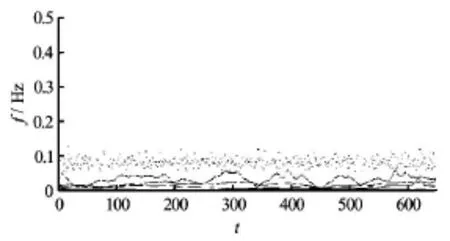
Fig.6 Hilbert spectrum

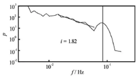
Fig.7 Hilbert marginal spectrum

2.4Analysis of Hilbert spectrum and Hilbert marginal spectrum

Figure 6 and Fig.7 show the Hilbert spectrum and the Hilbert marginal spectrum of monthly average temperature time series. They show that the energy is concentrated on the region of low frequency from 0.05 Hz to 0.1 Hz， and less energy is distributed on the region of higher frequency over 0.1 Hz， one sees the power law behaviour in the range 0.0144＜ω＜ 0.1074 month-1， with the scaling value of 1.82.

3. Conclusions

The analysis of the monthly average temperature time series by the HHT in Fengxian shows that the EMD method has a good adaptivityfor both nonlinear or linear cases. The relationship among the time，the frequency and the energy is obtained by the HHT，as follows：

（1） Through the EMD decomposing， the main change of the temperature follows the period of the annual variation， accompanying with several weaker oscillation periods. In recent 50 years， the change shows a falling →rising， →falling→rising trend.

（2） The analysis of the periods of each mode shows differrent variabilities of each mode， associated with a time scale almost twice as large as the time scale of the preceding mode.

（3） The analysis of the reconstructed modes of the wave pattern，shows that the variability is quite large from 1963 to 1964， from 1977 to 1982 and from 2003 to 2006， which indicates a dramatic temperature rising and falling in these periods. The volatility from 1993 to 1994 is far more dramatic than in other times. And it is the most remarkable in recent fifty years.

The Hilbert spectrum shows that the energy is concentrated on the region of low frequency from 0.05 Hz to 0.1 Hz， and less energy is distributed on the region of higher frequency over 0.1 Hz.

References

［1］SOLOMON S.， QIN D. and MANNING M. et al. IPCC：Climate change 2007-The physical scientific basis［M］. Cambridge， UK： Cambridge University Press，2007.

［2］ZHAO Zong-ci， WANG Shao-wu and XU Ying et al. Attribution of the 20th century climate warming in China［J］. Climatic and Environmental Research，2005， 10（4）： 807-817（in Chinese）.

［3］TANG Guo-li， REN Guo-yu. Reanalysis of surface air temperature change of the last 100 years over China［J］. Climatic and Environmental Research， 2005， 10（4）：791-798（in Chinese）.

［4］JI Fei， WU Zhao-hua and HUANG Jian-ping et al. Evolution of land surface air temperature trend［J］. Nature Climate Change， 2014， 4： 462-466（in Chinese）.

［5］BRAZDIL R.， CHROMA K. and DOBROVOLNY P. et al. Climate fluctuations in the Czech Republic during the period 1961-2005［J］. International Journal of Climatology， 2009， 29（2）： 223-242.

［6］GU Pin-qiang， WU Yong-qi. The climate change of forty years in Fengxian area and rational development and utilization of agriculture［J］. Journal of Agriculture Shanghai， 2000， 16（3）： 13-18（in Chinese）.

［7］GU Pin-qiang. Variation characteristic analysis of the first and last day of the four seasons in fengxian district of Shanghai for recent 50 years［J］. Atmospheric Science Research and Application， 2008， （2）： 107-112（in Chinese）.

［8］HUANG N. E.， CHERN C. C. and HUANG K. et al. A new spectral representation of earthquake data： Hilbert spectral analysis of station TCU129， Chi-Chi， Taiwan，21 September 1999［J］. Bulletin of the Seismological Society of America， 2001， 91： 1310-1338.

［9］CALIF R.，SCHMITTF. G. and HUANG Y. Multifractal description of wind power fluctuations using arbitrary order Hilbert spectral analysis［J］. Physica A： Statistical Mechanics and its Applications， 2013， 392（18）：4106-4120.

［10］VELTCHEVA A. D.， SOARE C. G. Identification of the components of wave spectra by the Hilbert Huang Transform method［J］. Applied Ocean Research， 2004，26（1-2）： 1-12.

［11］DUFFY D. G. The application of Hilbert-Huang Transforms to meteorological datasets［J］. Journal of Atmospheric and Oceanic Technology， 2004， 21（4）： 599-611.

［12］LU Zhi-ming， HUANG Yong-xiang and LIU Yu-lu. The analysis of an atmospheric turbulence data by Hilbert-Huang Transform［J］. Journal of Hydrodynamics， Ser. A， 2006， 21（3）： 310-317（in Chinese）.

［13］LEE Jeung-Hoon， HAN Jae-Moon and PARK HHyung-Gil et al. Application of signal processing techniques to the detection of tip vortex cavitation noise in marine propeller［J］. Journal of Hydrodynamics， 2013， 25（3）：440-449.

［14］SOURETIS G.， MANDIC D. P. and GRISSELI M. et al. Blood volume signal analysis with empirical mode decomposition［C］. 15th International Conference on Digital Signal Processing. Cardiff， UK， 2007， 147-150.

［15］HUANG Y.， SCHMITT F. G. Time dependent intrinsic correlation analysis of temperature and dissolved oxygen time series using empirical mode decomposition［J］. Journal of Marine Systems， 2014， 130： 90-100.

［16］HUANG Y.， SCHMITT F. G. Analysis of daily river flow fluctuations using empirical mode decomposition and arbitrary order Hilbert spectral analysis［J］. Journal of Hydrology， 2009， 373： 103-111.

［17］JIANG Zhi-hong， DING Yu-guo. Renewed study on the warming process of Shanghai during the past 100 years［J］. Quartely Journal of Applied Meteorology，1999， （2）： 155-156（in Chinese）.

［18］MU Hai-zhen， KONG Chun-yan and TANG Xu et al. Preliminary analysis of temperature change in Shanghai and urbanization impacts［J］. Journal of Tropical Meteorology， 2008， 24（6）： 673-674.

［19］SOURETIS G.， GRISSELI M. and TANAKA T. Blood volume signal analysis with empirical mode decomposition［C］. 2007 15th International Conference on Digital Signal Processing. Cardiff， UK， 2007， 147-150.

（December 12， 2014， Revised April 24， 2015）

* Project supported by the National Natural Science Foundation of China （Grant Nos. 11102114， 11172179 and 11332006）， the Inovation Program of Shanghai Municipal Education Commission （Grant No. 13YZ124）.

Biography： MA Hao （1989-）， Male， Master

QIU Xiang，

E-mail： emqiux@gmail.com