LI Dong-hui （李东晖）， XU Jing-yu （许晶禹）

LMFS， Institute of Mechanics， Chinese Academy of Sciences， Beijing 100190， China，E-mail： donghui_li@imech.ac.cn

Measurement of oil-water flow via the correlation of turbine flow meter， gamma ray densitometry and drift-flux model*

LI Dong-hui （李东晖）， XU Jing-yu （许晶禹）

LMFS， Institute of Mechanics， Chinese Academy of Sciences， Beijing 100190， China，E-mail： donghui_li@imech.ac.cn

The flow rate of the oil-water horizontal flow is measured by the combination of the turbine flow meter and the singlebeam gamma ray densitometry. The emphasis is placed on the effects of the pipe diameter， the oil viscosity and the slip velocity on the measurement accuracy. It is shown that the mixture flow rate measured by the turbine flow meter can meet the application requirement in the water continuous pattern （o-w flow pattern）. In addition， by introducing the developed drift-flux model into the measurement system， the relative errors of measurements for component phase flow rates can be controlled within ±5%. Although more accurate methods for the flow rate measurement are available， the method suggested in this work is advantageous over other methods due to its simplicity for practical applications in the petroleum industry.

oil and water flow， flow rate measurement， turbine flow meter， gamma ray densitometry， drift-flux model

Introduction

The simultaneous flow of two immiscible liquids is encountered in a diverse range of process industries. The measurement of the oil-water two-phase flow is one of the most critical technologies in the oil production. The flow rate of each component is measured without the need to separate each component in the two-phase flow. During the last decades， considerable efforts have been put in its studies for the oil and water flow， such as the developments of the V-cone flow meter， the single-phase meter， the ultrasonic techniques， the tomography and the capacitance probes［1］. Among these methods， the combination of two or more kinds of technologies makes a precise flow rate measurement possible. The measurement based on the correlation of a single phase flow meter with the densitometry becomes one of the main trends of current two phase flow measurements because of its simple structure and easy realization［2］.

The turbine flow meter is a kind of flow meters with good stability and high accuracy， which can work under the conditions of high temperature and high pressure. In recent years， the turbine flow meter was used to measure the mixture flow rate of a gas-liquid twophase flow［3］. In general， it is shown that the relative errors can be less than 20% in most cases when the gas fraction is small. However， little work has been reported in literature for the oil-water two-phase flow. For the mixture flow with a low oil volume fraction，the study of Skea and Hall［4］shows that the measurement errors could be controlled within 1% by using the turbine flow meter.

The component phase fraction is another parameter to be measured in order to estimate the flow rate of each phase. For the measurement of the local phase fraction， the electrical or optical local probes are used to obtain the dispersed phase fraction. Unfortunately，these two kinds of probes present the same types of shortcomings： the indirect measurement of the bubble size based on bubble chords and the low accuracy of the bubble parameters since the probes are localized in a limited portion of the pipe cross-section. These problems are partly solved by the use of wire-mesh sensors， which has been extensively applied in the gasliquid flow［5，6］and the oil-water flow［7］. However， dueto the different electrical conductivities of component phases， the method is limited to specific flow patterns based on continuous phases or dispersed phases. The gamma ray densitometry is a non-intrusive technique that does not disturb the flow under investigation， and is also simple for practical applications. Thus， this technique was successfully applied to the oil-water flow to obtain the local phase fraction under certain conditions［8］.

Fig.1 Schematic diagram of the oil-water two-phase flow loop

In order to extend the information gained from the measurements of the component phase flow rate in an oil-water horizontal flow， the present study uses the correlation of the turbine flow meter， the gamma ray densitometry and the drift-flux model. In the measurement system， the mixture flow rate is determined by a turbine flow meter and the component phase fraction is measured by a single beam gamma ray densitometry. Here， the gamma densitometry is installed in the necking pipe of 0.025 m in diameter since it is easier for the mixture flow to form a dispersed flow. In addition， the drift-flux model is developed to identify the phase velocity according to the effects of the slip velocity on the measurement. Based on the experimental data， the measurement accuracy can be improved greatly and the prediction errors are less than 5%.

1. Experimental system

A schematic diagram of the experimental system is shown in Fig.1. All experiments are conducted by using white oils with two different viscosities and water at room-temperature and under atmospheric outlet pressure. The system consists of a steel frame supporting a transparent Perspex pipes. Water and oil are pumped from their respective storage tanks， metered， and introduced into pipes via a T-junction. The volumetric flow rates of two phases could be regulated independently and are measured by a root flow meter （LLQ） for oil phase and an electromagnetic flow meter for water phase， respectively. The mixture flows along a 14 m long horizontal pipe from the entry point to the test section， which provides a sufficient entrance length to stabilize the flow. The flow regimes are determined based on visual observations，and a high-speed camera and a still picture camera are used to visualize the flow.

1.1Single-beam gamma densitometry

In this work， the densitometer is equipped with a radioactive source， a detector and a signal processing system. The source and the detector are located diametrically opposite to each other on the test section. The source is mounted inside a lead shielding container. The gamma densitometer is installed in the middle of the test tube， to measure the gamma ray absorption， which allows the local phase fraction to be calculated. The densitometer is calibrated by scanning a Plexiglass box which contains water and oil in different ratios and thus provides different phase fraction values to be used as calibration points. The counting rate is integrated over 80 energy bands centered at the peak energy band of the 662 keV generated from the 137 Cs scattering. The gamma counts are recorded for three separate periods of 60s to obtain an average value of the phase fraction， with a measurement error of 6.12%.

To check the data from the gamma densitometer，the average local phase fraction is also measured by two rapid closing valves， which are the full opening ball valves with an inside diameter equal to the inside diameter of the pipe so that the flow is not disturbed by passing through the open valves. The two rapid closing valves connected by mechanical linkages are installed in the test section at a distance of 1 m. The operation time of the two rapid closing valves is 0.5 s. This provides a sufficient short time to measure accurately the phase volumes. During the average local phase fraction measurement runs， a sufficient time is taken to allow the establishment of a fully developed flow. The rapid closing valves are closed to get a representative sample of two-phase flows. The sample is then transferred to a graduated cylinder by carefullypurging the liquid phases using pressurized gas in order to assure not to leave any liquid inside of the test section. The samples are left in graduated cylinders for a time period of about 6 h to assure virtually complete gravitational phase separation before the measurement of the liquid phase volumes. By taking repeated measurements of samples it is found that the fluctuation of the mean value of the measurements over the three runs is around 6.7%.

1.2Turbine flow meter

Turbine flow meters are frequently used in the measurement of single-phase flow rates. In principle，the turbine meter operates simply as a hydraulic turbine. It is essentially a device which rotates as the fluid flows through the turbine blades， and the rotational speed of the blades is related to the volumetric flow rate. In a single-phase flow， the fluid passes through the pipe and drives the turbine rotation. The relationship between the rotate speed of the turbine and the flow rate is as follows

whereQ is the volume flow rate，fthe rotating speed of the turbine andKthe meter factor， which may be influenced by the fluid properties. The measurement uncertainty will increase when the second phase component is present in the turbine flow meter. Therefore， both the input oil fraction and the oil viscosity can affect the measurement precision of the turbine flow rate when it is used in two-phase flows. In the present study， the LWGY turbine flow meters with nominal diameter of 0.050 m and 0.025 m， respectively， are used to measure the mixture flow rate in the range of 2 m3/h-40 m3/h. For a single-phase water flow， the measurement accuracy is 0.5%. The relative error of the turbine flow meter is defined as

1.3Test matrix

One of the main goals of the experimental work is to generate a comprehensive set of data in oil and water flows. Thus， the ranges of oil and water flow rates covered are 0 m3/h-13 m3/h and 0 m3/h-15 m3/h，respectively. To examine the effect of the diameter on the measurement of the local phase fraction， the test sections of the two different pipes are 0.05 m and 0.025 m in diameter， respectively. Moreover， the influences of the fluid viscosity on the turbine flow meter are also considered by using two kinds of while oils of different viscosities. The physical properties of test liquids are listed in Table 1.

Table 1 Liquid phase's properties measured at 20oC and 0.101 MPa

2. Theory

2.1Component phase flow rate by the homogenized model

The mixture flow rate of the oil-water flow， measured by using the turbine flow meter， is defined as

where the subscripts o and w refer to the oil phase and the water phase， respectively. The component phase flow rates can be given， respectively， as：

where A is the pipe cross-sectional area and uthe average velocity.εois the average local oil phase fraction. If the mixture flow is homogenized before being measured， it can be assumed that a no-slip condition is prevailed between the phases. The component phase velocity is equal to the mixture velocity

then， once a solution is obtained for εoby the singlebeam gamma densitometry， the component phase flow rates can be obtained， respectively， as：

2.2 Component phase flow rate by the drift-flux model

In fact， due to the different densities of the two fluids， for different local phase fractions， there is a slip velocity between two phases under most of inlet conditions. Namely， it is impossible that two component phase velocities are equal. In general， the slip phenomenon can be expressed in terms of the ratio between the average local velocities of the two-phases， with S being defined as the ratio of the local oil to water velocities， as follows

whereβis the input phase volume fraction. Accordingly，S is greater than 1 when the oil is the faster flowing phase， and conversely，S is less than 1 when the water is the faster flowing phase.

For a two-phase mixture flow， two available methods， the two-fluid model and the drift-flux model，are commonly used to predict the component phase velocity. In the two-fluid model， the liquids are treated as completely separated layers with a smooth interface，which， in most cases， will lead to an underestimation of the measurements［9，10］. Thus， the drift-flux model is considered as advantageous over other methods due to its simplicity and enough accuracy to be practically applied in industry. In the present work， the drift-flux model， which modifies the homogeneous flow theory to account for the slip velocity between oil and water，is used to predict the oil velocity as

where C0describes the effects of the non-uniform distribution of both velocity and concentration profiles. If oil and water are uniformly mixed， the concentration profile will be flat andC0should be equal to unity.udis called the drift velocity， and accounts for the local relative velocity between two phases. If the liquid is stationary，udcorresponds to the rise velocity of the dispersed phase in the stagnant liquid. Traditionally， the drift-flux model is used most widely for vertical dispersed systems， and it is derived from the continuity equation in dispersed systems［11］. The model is extended to include the segregated horizontal flows［12，13］. In Fig.6，uovs.umcurves are plotted in two different flow patterns. By using the linear regression， the two parameters C0and udcan be determined.

By substituting Eq.（10） into Eqs.（3） and （4）， the component phase flow rates can be expressed， respectively， as：

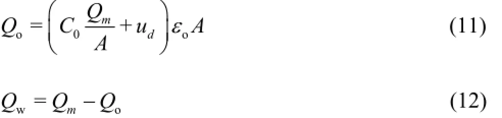
Fig.2 Relative error vs. input oil fraction with oil viscosities of 50 mPa·s and 138 mPa·s， respectively

3. Results and discussions

3.1Mixture flow rate by the turbine flow meter

The relative error vs. the input oil fraction curves are shown in Figs.2（a） and 2（b） for the oil-water flow with oil viscosities of 50mPa·s and 138mPa·s， respectively. Most of data are obtained from measurements in the dispersed flow regimes. It can be seen that the errors increase slightly with the increase of the input oil fraction and then decrease sharply around the phase inversion region. Based on our previous studies［13］， for the mixture flow of white oil and water the point of phase inversion is always close to the range of the input oil fraction from 0.7 to 0.8. Thus， it is interesting that the relative errors are always positive when the mixture flowing in the water continuous pattern （o/w flow pattern）. On the other hand， most of the relative errors are negative for the oil continuous flow （w/o flow pattern）， and this means that the measurement values are always less than the actualvalue. Moreover， the absolute values of the relative errors of the latter are significantly greater than those of the former. This phenomenon is consistent with the findings of Huang et al.［14］.

In this work， the relative error of ±5%is defined as the standard to define the valid work area［15］，and two horizontal lines of the relative error of ±5% is used to distinguish the effective boundary of the work area. It can be found in Fig.2（a） that for the mixture flow with oil viscosity of 50 mPa·s， the relative errors are within ±5%during the entire range and the turbine flow-meter works well at any given oil fraction. However， for the mixture flow with oil viscosity of 138 mPa·s， Fig.2（b） shows that the absolute value of the relative errors keep within 5% in the water continuous pattern. With the input oil fraction increasing，the errors sharply decline and go bellow -5%. The failure area appears in the range of 0.8-1 of the input oil fraction. This phenomenon is probably due to the fact that there is a certain dependence of parameterK in Eq.（1） on the Reynolds number. Here， the parameter is assumed as constant based on the low viscosity fluid. Therefore， the errors could be enlarged in the oil continuous pattern since the apparent viscosity of the fluids is affected mainly by the viscosity of a continuous phase.

In general， the experiment results indicate that the valid work area of the turbine flow meter is influenced by both the oil viscosity and the input oil fraction. Under the condition of a high viscosity oil， the unacceptable turbine flow-meter errors appear in the oil continuous pattern. If the ±5%accuracy limit is acceptable in industrial applications， the mixture flow with a low viscosity oil can meet the requirements of the turbine flow meter applications for the entire range of oil fraction， and yet for the high viscosity oil-water flow， the turbine flow meter could be suggested to measure the mixture flow rate in the water continuous patterns. These data are in accord with those of Guo et al.［16］.

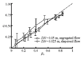
Fig.3 Local oil fraction versus input oil fraction by using the gamma densitometry with two different pipe diameters

3.2Local oil fraction by the gamma ray densitometry

Figure 3 depicts the local oil fraction vs. the input oil fraction curves by using the gamma densitometry with two different pipe diameters. Here， the actual local oil fractions are measured by the repaid closing valves. Although all test points are obtained by two methods for the local oil fractions， only selected one constant mixture flow rate is included in the Figure. It can be found that the data by the gamma densitometer in the 0.050 m diameter case show a large deviation from the actual values. Based on experimental observations， when the mixture flow rate is 4.5 m3/h， the oil-water flow pattern in the 0.050 m diameter case is a segregated flow， while the pattern in the 0.025 m diameter case is a dispersed flow.

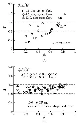
Fig.4 Ratio of local oil to water velocity versus input oil fraction at constant mixture flow rates， respectively， with two different pipe diameters

Figure 4 shows the effects of the pipe diameter and the flow pattern on the slip velocity at constant input mixture flow rates. Most flow patterns in 50 m diameter pipes are a segregated flow. On the other hand， those in the 0.025 m diameter pipes are a dispersed flow. In Fig.4（a）， for two constant mixture flow rates （2.0 m3/h and 4.5 m3/h）， the velocity ratio（）S increases quickly from 0.3 to 1.6 with the input oil fraction increasing. However， for those in the 0.025 m diameter pipes， the velocity ratio is less sensitive to thethe input oil fraction， and all data points are in a band between 0.8 and 1.2. Thus， combined with Fig.3， the test section with a small diameter is more appropriate to obtain the local phase fraction by the single-beam gamma densitometer.

Fig.5 Comparison of the component phase flow rates predicted with input oil or water flow rates under the condition of no-slip assumption

3.3Component phase flow rate

Under the no-slip condition between the phases，Fig.5 shows a comparison of the component phase flow rates， predicted by the homogenized model， with the input oil or water flow rate for the mixture flow in the 0.025 m diameter case. It can be seen that the results predicted by the correlation of a turbine flow meter with the gamma ray densitometry enjoy a reasonably good performance with 90% of the data falling in the range of ±20%. However， a more accurate prediction of the flow rates should be possible if the slip velocity is considered. Thus， in the following prediction， the slip velocity is introduced into the measurement system by using the drift-flux model.

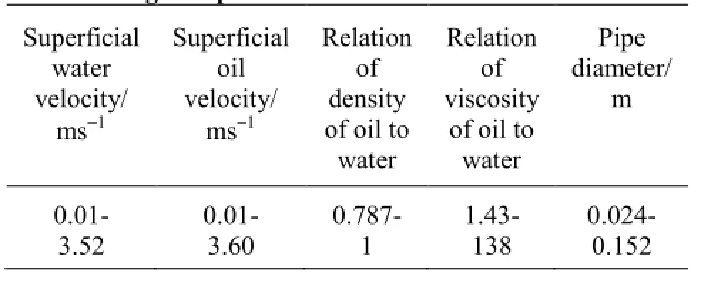
Table 2 Ranges of parameters in collected data

To resolve C0and udin Eq.（10）， the drift-flux model is used to determine the slip velocity. Here， the flow patterns are classified into the following two categories［17］： the segregated flow， where the two fluids flow in separate layers according to their different densities （ST or ST and MI flows）， and the dispersed flow， where one fluid is continuous and the other is in the form of drops dispersed in it （Do/w and w，Dw/oando，Do/wandDw/o，o/worw/o flows）. About 685 experimental data points are collected， and the range of parameters are given in Table 2. The experimental data consist of the hydraulic pipe diameters in a range from 0.024 m to 0.152 m， and the oil phase viscosities from 1.43 mPa·s to 138 mPa·s［9，18-24］. The correlation calculation related to the two systems can be used to establish the following function：

Fig.6 Correlation coefficients calculated referring to the corresponding set of experimental data in this work and for other systems reported in literature

The comparisons of the theoretical predictions obtained from Eqs.（13） and （14） for the average local oil velocity with experimental data in this work and for other systems reported in literature are shown in Fig.6. It can be seen that a good agreement is obtainedbetween theory and data. The fitting results are within the average absolute error of 6.03% for the dispersed flow and 8.05% for the segregate flow， respectively. These results substantiate the general validity of the models presented for predicting the average local oil velocity when the flows are divided into two different categories. By substituting Eqs.（13） and （14） into Eqs.（11） and （12）， Fig.7 illustrates the comparison of the predicted component phase flow rates with the input oil or water flow rates. It can be observed that the predicted results can describe the majority of the experimental data within ±5%of errors. The comparison with Fig.6 shows that this improvement enhances the prediction precision.

4. Conclusions

The present study measures the flow rates in an oil-water flow via the correlation of the turbine flow meter， the gamma ray densitometry and the drift-flux model. Based on the experimental results and analysis，the following conclusions can be reached：

When the turbine flow meter is used to measure the mixture flow rate of oil and water， the mixture flow with low viscosity oil can meet the requirements of the turbine flow meter applications for the entire range of oil fraction， and yet for high viscosity oil and water flow， the turbine flow meter is suggested to measure the mixture flow rate in thewater continuous patterns. The single-beam gamma densitometry installed in the pipe of small diameter is more appropriate to obtain the local phase fraction since the mixture flow is easier to form the dispersed flow.

Measurements of the component phase flow rates by the correlation of a turbine flow meter with the gamma ray densitometry enjoy a reasonably good performance with 90% of the data falling in the range of ±20%. However， by introducing the developed driftflux model into this combination instrument， the measurement accuracy can be improved greatly， and the prediction errors are less than±5%. Although more accurate methods for the flow rate measurements of the oil-water flow might be applied， the method suggested in this work is advantageous over other methods due to its simplicity for practical applications in the petroleum industry.

References

［1］FALCONEG.，HEWITT G. F. and ALIMONTIC. Multiphase flow metering： principles and applications［M］. London， UK： Elsevier， 2009.

［2］ZHENG G.， JIN N. and JIA X. et al. Gas-liquid two phase flow measurement method based on combination instrument of turbine flowmeter and conductance sensor［J］. International Journal of Multiphase Flow，2008， 34（11）： 1031-1047.

［3］MINEMURA K.， EGASHIRA K. and IHARA K. et al. Simultaneous measuring method for both volumetric flow rates of air-water mixture using a turbine flowmeter［J］. Journal of Energy Resources Technology，1996， 118（1）： 29-35.

［4］SKEA A. F.， HALL A. W. Effects of water in oil and oil in water on single-phase flowmeters［J］. Flow Measurement and Instrumentation， 1999， 10（3）： 151-157.

［5］OLERNI C.， JIA J. and WANG M. Measurement of air distribution and void fraction of an upward air-water flow using electrical resistance tomography and wiremesh sensor［J］. Measurement Science and Technology， 2013， 24（3）： 035403.

［6］LUCAS D.， KREPPER E. and PRASSER H. M. Development of co-current air-water flow in a vertical pipe［J］. International Journal of Multiphase Flow，2005， 31（12）： 1304-1328.

［7］RODRIGUEZ I. H.， YAMAGUTI H. K. B. and De CASTRO M. S. et al. Slip ratio in dispersed viscous oilwater pipe flow［J］. Experimental Thermal and Fluid Science， 2011， 35（1）：11-19.

［8］KUMARA W. A. S.， HALVORSEN B. M. and MELAAEN M. C. Single-beam gamma densitometry measurements of oil-water flow in horizontal and slightly inclined pipes［J］. International Journal of Multiphase Flow， 2010， 36（6）： 467-480.

［9］ANGELI P.， HEWITT G. F. Flow structure in horizontal oil-water flow［J］. International Journal of Multiphase Flow， 2000， 26（7）： 1117-1140.

［10］XU J.， WU Y. and FENG F. F. et al. Experimental investigation on the slip between oil and water in horizontal pipes［J］. Experimental Thermal and Fluid Science， 2008， 33（1）： 178-183.

［11］GOVIER G. W.， AZIZ K. The flow of complex mixtures in pipes［M］. New York， USA： Van Nostrand Reinhold Company， 1972.

［12］FRANCA F.， LAHEY Jr R. T. The use of drift-flux techniques for the analysis of horizontal two-phase flows［J］. International Journal of Multiphase Flow，1992， 18（6）： 887-801.

［13］XU J.， WU Y. and CHANG Y. et al.. Experimental investigation on the holdup distribution of oil-water twophase flow in horizontal parallel tubes［J］. Chemical Engineering and Technology， 2008， 31（10）： 1536-1540.

［14］HUANG Z.， LI X. and LIU Y. et al. Experimental study on performance of turbine flowmeter and venturi meter in oil water two phase flow measurement［C］. AIP Conference Proceedings， 2007， 914（1）： 678-682.

［15］YE B. New progress in multiphase metering technology［J］. Foreign Oilfield Engineering， 2010， 26（2）： 52-54（in Chinese）.

［16］GUO S.， SUN L. and ZHANG T. et al. Analysis of viscosity effect on turbine flowmeter performance based on experiments and CFD simulations［J］. Flow Measurement and Instrumentation， 2013， 34： 42-52.

［17］XU J.， LI D. and GUO J. et al. Investigations of phase inversion and frictional pressure gradients in upward and downward oil-water flow in vertical pipes［J］. International Journal of Multiphase Flow， 2010， 36（11-12）： 930-939.

［18］CHARLES M. E.， GOVIER G. W. and HODGSON G. W. The horizontal pipeline flow of equal density oilwater mixtures［J］. The Canadian Journal of Chemical Engineering， 1961， 39（1）： 27-36.

［19］LOVICK J.， ANGELI P. Experimental studies on the dual continuous flow pattern in oil-water flows［J］. International Journal of Multiphase Flow， 2004， 30（2）：139-157.

［20］ODDIE G.， SHI H. and DURLFOSKY L. J. et al. Experimental study of two and three phase flows in large diameter inclined pipes［J］. International Journal of Multiphase Flow， 2003， 29（4）： 527-558.

［21］RAJ T. S.， CHAKRABARTI D. P. and DAS G. Liquidliquid stratified flow through horizontal conduits［J］. Chemical Engineering and Technology， 2005， 28（8）：899-907.

［22］RODRIGUEZ O. M. H.， OLIEMANS R. V. A. Experimental study on oil-water flow in horizontal and slightly inclined pipes［J］. International Journal of Multiphase Flow， 2006， 32（3）： 323-343.

［23］RUSSEL T. W. F.， HODGSON G. W. and GOVIER G. W. Horizontal pipeline flow of mixtures of oil and water［J］. The Canadian Journal of Chemical Engineering， 1959， 37（1）： 9-17.

［24］TRALLERO J. L.， SARICA C. and BRILL J. P. A study of oil/water flow patterns in horizontal pipes［J］. SPE Production and Facilities， 1997， 12（3）： 165-172.

（October 7， 2014， Revised January 13， 2015）

* Project supported by the National Key Scientific Instruments in China （Grant No. 2011YQ120048-02）.

Biography： LI Dong-hui （1962-）， Male， Senior Engineer

XU Jing-yu，

E-mail：xujingyu@imech.ac.cn