Sisira Ediriweera · Sumith Pathirana ·Tim Danaher Doland Nichols

ORIGINAL PAPER

Estimating above-ground biomass by fusion of LiDAR and multispectral data in subtropical woody plant communities in topographically complex terrain in North-eastern Australia

Sisira Ediriweera · Sumith Pathirana ·Tim Danaher Doland Nichols

Received: 2013-02-12 Accepted: 2013-10-31

© Northeast Forestry University and Springer-Verlag Berlin Heidelberg 2014

We investigated a strategy to improve predicting capacity of plot-scale above-ground biomass (AGB) by fusion of LiDAR and Landsat5 TM derived biophysical variables for subtropical rainforest and eucalypts dominated forest in topographically complex landscapes in North-eastern Australia. Investigation was carried out in two study areas separately and in combination. From each plot of both study areas, LiDAR derived structural parameters of vegetation and reflectance of all Landsat bands, vegetation indices were employed. The regression analysis was carried out separately for LiDAR and Landsat derived variables individually and in combination. Strong relationships were found with LiDAR alone for eucalypts dominated forest and combined sites compared to the accuracy of AGB estimates by Landsat data. Fusing LiDAR with Landsat5 TM derived variables increased overall performance for the eucalypt forest and combined sites data by describing extra variation (3% for eucalypt forest and 2% combined sites) of field estimated plot-scale above-ground biomass. In contrast, separate LiDAR and imagery data, andfusion of LiDAR and Landsat data performed poorly across structurally complex closed canopy subtropical rainforest. These findings reinforced that obtaining accurate estimates of above ground biomass using remotely sensed data is a function of the complexity of horizontal and vertical structural diversity of vegetation.

Fusion, above-ground biomass, LiDAR, multispectral data, subtropical plant communities

Introduction

Forest ecosystems exert considerable influence on global carbon cycles through the flux and storage of carbon in plant biomass (Chave et al. 2005). Plant biomass in forests is distributed above and below ground, and is the total amount of biological material present above the soil surface in a specified area. Tree biomass is useful, for example, in assessing forest structure and condition (Westman et al. 1977; Specht et al. 1999), to estimate forest productivity and carbon fluxes based on sequential changes in biomass (Chambers et al. 2001) to provide a means of assessing sequestration of carbon in wood, leaves, and roots (Specht and West 2003), and also as an indicator of both the biological and economic value of a forest ecosystem. Thus, estimation of forest biomass at different geographical scales (from local to global) becomes significant in reducing uncertainty of carbon emission and sequestration, understanding its role in influencing soil fertility, measures of land degradation or restoration, and understanding the roles a forest plays in environmental processes and sustainability (Foody et al. 2003).

Remotely sensed data such as Light Detection and Ranging (LiDAR) and multispectral satellite data can be effectively used to estimate above-ground biomass (AGB) of forested landscapes. With the increasing availability of multispectral space-borne high resolution systems in recent years interest rose on estimation offorest biomass in small scale and landscape scale in natural and plantation forests (Foody et al. 2001, Lu and Batistella 2005 ). Additionally, LiDAR has proven to have potential to estimate AGB at individual tree level (Bortolot et al. 2005; Popescu 2007) and at plot- scale (Riggins et al. 2009; Latifi et al. 2010). Advantages of estimating biomass using remote sensing include the ability to obtain measurements from any location in a forested area, the speed with which remotely sensed data can be collected and processed, the relatively low cost of various remote sensing data, and the ability to collect data easily in extensive areas containing diverse topography.

In order to estimate AGB of structurally complex subtropical rainforest and eucalypt forest in rugged terrain, this study is focused on both LiDAR and Landsat5 TM data. It is assumed that combination of LiDAR and Landsat data gain strength of both technologies which will improve predictions of AGB on areas influenced by topographic and microclimatic variations in complex forests. LiDAR represents one of the best sources of information for investigating vegetation structural parameters (e.g. tree height, crown area, foliage cover) and provides detailed information on vertical profiles of vegetation. Landsat-data is a powerful source of data on spectral information of land use and landcover, allowing the detection of vegetation structure and structural changes in the vegetation. There have been a number of studies examining the fusion technique to estimate plot-scale forest volume and biomass integrating small foot print LIDAR with multispectral satellite data in deciduous and pine forests (Popescu et al. 2004). Similarly Latifi et al. (2010) estimated timber volume and biomass using a non-parametric method in a temperate forest combining LiDAR and Landsat data. Tonolli et al. (2011) combined LiDAR with IRS 1C LISS III derived biophysical variables to estimate plot-scale timber volume in the Southern Alps. Hudak et al. (2006) integrated LiDAR and multispectral data to model and map basal area and tree density across two diverse coniferous forests. Additionally, Jensen et al. (2008) improved LiDAR based plot-scale Leaf Area Index (LAI) quantifying capacity by adding SPOT derived vegetation indices.

In general, estimation of AGB in structurally complex tropical and subtropical forests, much uncertainty remains regarding estimation accuracy (Lu et al. 2012). Furthermore, estimation of the plot-scale AGB of tropical and subtropical forests in topographically complex terrain has been poorly investigated. We assumed that employment of data fusion would improve estimation of plotscale AGB as it comprises vertical and horizontal information of vegetation structure derived from LiDAR and multispectral data even in areas such as structurally complex vegetation on rugged topography. The purpose of this study is to improve the capacity of estimating plot-scale AGB for eucalypt dominated forest and subtropical rainforest by fusion of small footprint LiDAR and Landsat5 TM multispectral data. The study translates into two more targeted objectives: (1) the capability of LiDAR derived structural parameters of vegetation (LiDAR variables) and Landsat5 TM variables to estimate measured plot-scale AGB, and (2) the extent to which combining of Landsat5 TM and LiDAR derived variables may improve estimates of AGB in topographically dissected landscape. A unique characteristic of this vegetation is the floristic variation in relation to the changes in topography by distributing sclerophyll forests (eucalypt dominated), particularly on the ridges or upper slopes, and subtropical rainforests restricted to the gullies or lower slopes (Florence 1996). Therefore, data were analysed in both plant communities separately and in combination.

Material and methods

Study areas

Two study areas were located in New South Wales (NSW), Australia (Fig. 1) including the Richmond Range National Park (RRNP) (28.69º S, 152.72º E) and the Border Ranges National Park (BRNP) (28.36º S, 152.86º E). The elevation of RRNP study area ranges from approximately 150 m to 750 m above mean sea level with an average slope of 27º. Annual rainfall is approximately 1200 mm and the average temperature ranges in the winter is 12–21 °C and 25–31 °C in the summer (Bureau of Meteorology 2010).

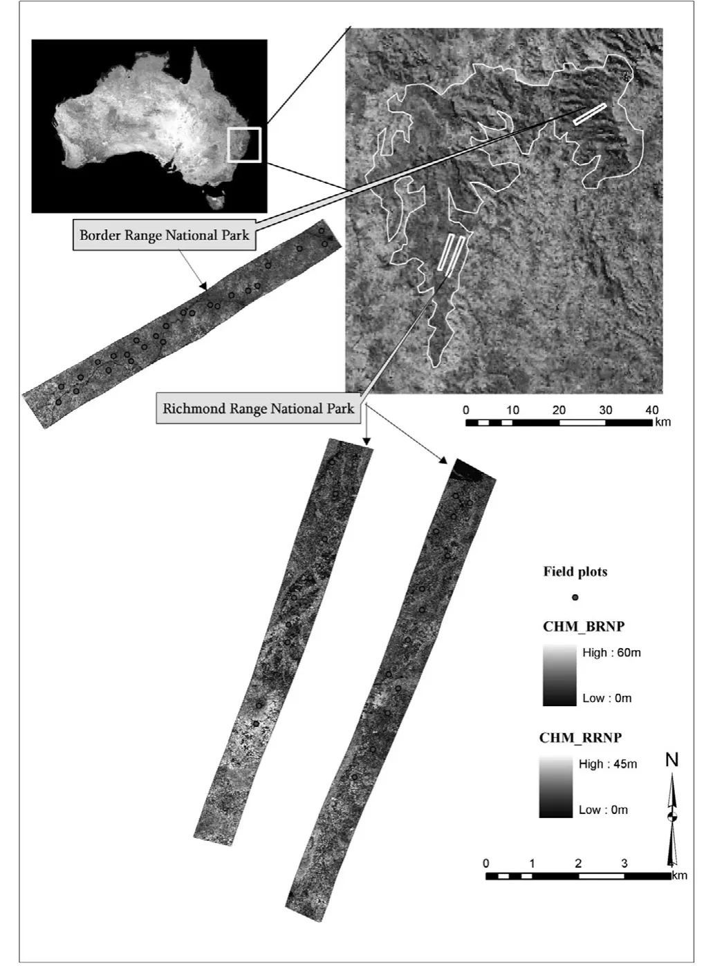
Fig. 1: Location map of the Border Range National Park and the Richmond Range National Park plots and LiDAR acquisition areas, New South Wale

The RRNP is an open canopy eucalypt-dominated forest with 30%–70% Foliage Projective Cover (FPC). The Foliage Projective Cover is defined as the vertically projected percentage coverof photosynthetic foliage of all strata (Specht et al. 1999). In order of dominance by per cent basal area eucalypts species found in the RRNP, include Corymbia maculata, Eucalyptus propinqua, E. siderophloia, and Lophostemon confertus. The understorey is mainly covered by native grass and shrub species. The elevation of the BRNP study area ranges from approximately 600 m to 1200 m above mean sea level with an average slope of 36°. Annual rainfall is approximately 3000 mm, and the average temperature ranges 3–19 °C in the winter and 15–31 °C in the summer (Bureau of Meteorology 2010). The BRNP is a tall closed canopy subtropical rainforest with 70%–100% FPC (Specht et al. 1999). The most common species based on proportional basal area are Planchonella australis, Heritiera actinophylla, Sloanea woollsii, Geissois benthamiana and Syzygium crebrinerve (Smith et al. 2005). Both study areas are managed by the NSW Office of Environment and Heritage.

Field data collection

Field sampling was conducted between July and December 2010. There were 50 sample plots representing 25 plots of 50 m × 50 m (0.25 ha) for each study area were randomly selected within each LiDAR transect across the two forested areas. A random sampling method was adopted to assure that sampling measurements acquired all possible variability of forests conditions. The centre of each plot was determined by using a GPS unit (GARMIN GPSMAP (R) 62stc). Five GPS points were collected in the centre of each plot over a 20 minute period and then averaged. The accuracy of the GPS varied with the density of overstorey with standard deviation of the five measurements ranging from 5 m to 8 m in the closed canopy BRNP and from 3 m to 6 m in the open canopy RRNP.

Dbh (1.3 m height) was measured for all trees in each plot in both study areas using a diameter tape with diameters for buttressed trees measured immediately above the buttress. Tree height and crown width for all trees which were larger than 10 cm dbh were separately measured in selected five plots of each study area. Tree heights were measured using a Nikon Forestry 550 Laser Rangefinder/ Heightmeter. A SUUNTO clinometer was used to delineate tree crowns by vertically upward sighting and taking averages value of four perpendicular crown radii measurements with a distance tape from the tree trunk towards the plot centre, away from it, to the right and to the left.

Above-ground biomass estimation

Above-ground biomass was estimated based on previously developed allometric equations of plant communities in Australia. Two general allometric equations were considered (Keith et al. 2000) as equations at finer taxonomic resolution were not available for the specific vegetation types found in the study area. For subtropical rainforest:

For open canopy eucalypts forest:

where Y = AGB (kg), X = dbh (cm).

Table 1 shows a summary of statistics of the estimated AGB of both study areas using allometirc equations.

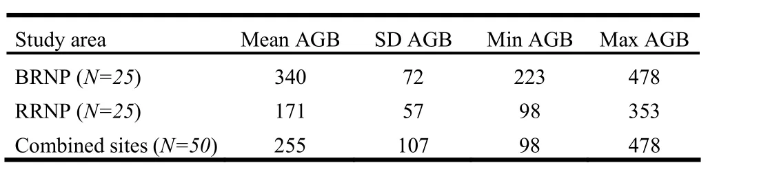
Table 1: Basic statistics of the estimated AGB (t/ha) of both study areas

LiDAR data

LiDAR data were collected during July and August 2010 using a Leica ALS50-II LiDAR system at a flying height of 2000 m. The laser pulse repetition frequency was 109 kHz. The laser scanner was configured to record up to four returns per laser pulse. The average point density (i.e. number of LiDAR points collected within a square meter) was 1.3 points per square meter, and the footprint diameter was 0.5 m. The average range varied between 524 m and 1018 m (mean 800 m) for the BRNP and 157 m and 460 m (mean 256 m) for the RRNP. The mean rates of penetration (the percentage of laser beams penetrating to a specific height class is defined with the rate of laser beam penetration) through the vegetation vary from 4.3% in the closed canopy of BRNP and 19% open canopy of RRNP. The LiDAR data were documented as 0.07 m for vertical accuracy and 0.17 m for horizontal accuracy by the data provider. The LiDAR data were classified into ground and non-ground points using proprietary software by the NSW Land and Property Information (LPI) and were delivered in LAS 1.2 file format.

Multispectral data

Cloud and haze free Landsat5 TM data were captured on 15 October 2011 under high sun angle conditions (54.6o). Landsat5 TM (Level 1 G), product (Path/Row– 89/80) was acquired from the United States Geological Survey (USGS). The Landsat5 TM image was obtained from the USGS as rectified data in universal transverse mercator projection at 30 m resolution. Radiometric calibration of the Landsat5 TM image was a procedure containing multi-steps. Firstly, the 8-bit satellite digital numbers (DN) in Landsat5 TM image were converted to at-satellite radiance using the most recent calibration coefficients (Markham et al. 2012). Next the top-of-atmosphere radiance was converted to surface reflectance. The Second Simulation of the Satellite Single in the Solar Spectrum atmospheric radiative transfer modelling (6S), a generic model (Vermote et al. 1997) was used to predict the direct and diffuse irradiance from clear sky onto horizontal surfaces withan Aerosol Optical Depth (AOD) of 0.05 for this study. A bi-directional reflectance model correction was applied to remove the effects of angular variation in reflectance due to varying sun and view angles (Flood et al. 2012). The processing scheme for standardised surface reflectance was employed to minimise the topographically induced illumination.

Data processing

Fig. 2 shows a flowchart of the processing steps carried out in this study. A detailed description of the steps is presented in the following section.

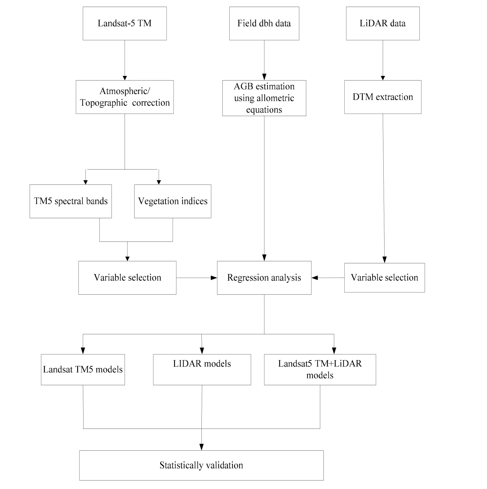
Fig. 2: Flowchart of the model building method

LiDAR data pre-processing

All returns were considered for subsequent analysis for both study areas. Ground and non-ground returns were separated and a 1m Digital Terrain Model (DTM) was produced using ground returns via Kriging interpolation to the nearest 6 data points. The accuracy of LiDAR-derived DTM was evaluated using seventy and fifty five post-processed differential GPS points (dGPS) for the BRNP and RRNP respectively. The GPS points collected using a MobileMapper from Thales Navigation (TM) systems and included 4 transects for the BRNP and 3 for the RRNP. Collected GPS points were distributed over flat to slope terrain in open ground (park roads) and under forest canopies in different densities. The calculated root mean square errors (RMSE) were 5.7 m and 1.9 m for the closed canopy BRNP and open canopy RRNP respectively.

Computation of LiDAR metrics

LiDAR metrics were calculated from separated non-ground laser returns. Observations with height values ＜2 m for the RRNP and＜0.5 m for the BRNP were discarded from existing non-ground data in order to remove undulation of the terrain and other objects (herbaceous vegetation, fallen logs etc.). Thus, most reflectance would correspond to understorey and overstorey vegetation. The non-ground returns was used to extract co-located 50 m x 50 m field sample plots of each study area and subsequently a series of LiDAR metrics were computed.

(1) The calculated height related LiDAR metric for individual sampling plots include maximum, mean, median and relative median canopy height and from 10thto 90thheight percentiles.

(2) LiDAR fractional cover is defined one minus the gap fraction probability at a zenith of zero (Lovell et al. 2003) which corresponds to the photosynthetic and non-photosynthetic components of canopy. Fractional cover was calculated by aggregating all points into 50 m spatial bins using equation 1

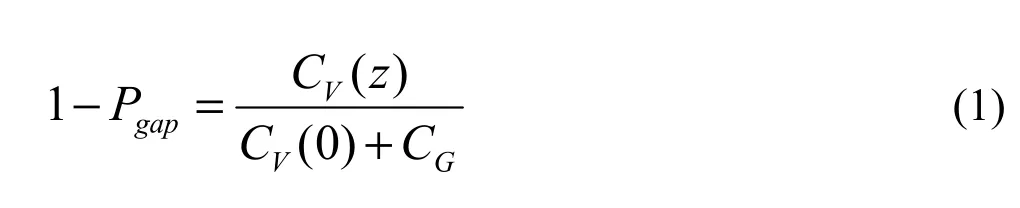
where Cv(z) is the number of first returns counts above Z meters, Cv(0) is the number of first returns above the ground and CGwas the number of first return points from the ground level.

(3) Tree crown diameter was estimated on the LiDAR derived 1 m resolution canopy height models (CHM) using non-ground laser returns by TreeVaw 1.1 software (Popescu et al. 2003). The derivation of the appropriate window size to search for tree tops is based on the relationship between the height of the trees and their crown size (Popescu et al. 2003). In order to derive the appropriate window size to search for tree tops, field measured tree heights and crown widths were separately used to develop a relationship for both forest types. As Popescu et al. (2003) explained CHM based tree crown diameter estimation is more appropriate to measure crown diameter for dominant and co-dominant trees that have individualized crowns on the CHM surface. Average crown diameters of each sample plot were estimated at several canopy heights; 15 m, 20 m, and 30 m for RRNP and 15 m, 20 m and 35 m for BRNP. LiDAR derived heights, fractional cover and crown diameter variables corresponding to the sampling sites are summarised in Table 2.

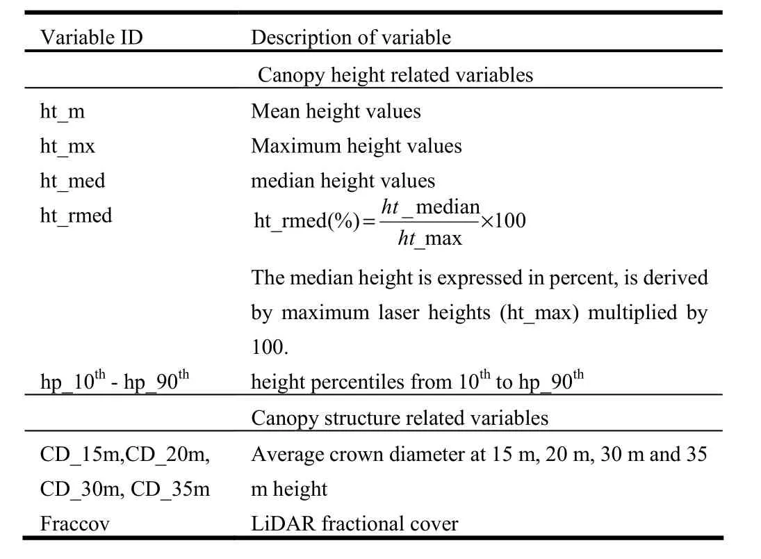
Table 2: Variables computed from LiDAR returns in each study area

Computation of Landsat5 TM variables

Signatures for Landsat5 TM bands were extracted for the 2 × 2 pixel mean surrounding the field site location. The 2 × 2 block average provided the best match to the spatial extent of field measurements and also minimized the effects of geometric misregistration between imagery of different dates. It was assumed that any increase in vegetation structure between the date of site measurement and the image acquisition date was less than measurement error, as sites were generally located in mature vegetation. Proposed Landsat5 TM variables included: (1) normal band values, (2) simple band ratios, (3) normalized band rations, and (4) high order transformed greenness indices (Table 3).

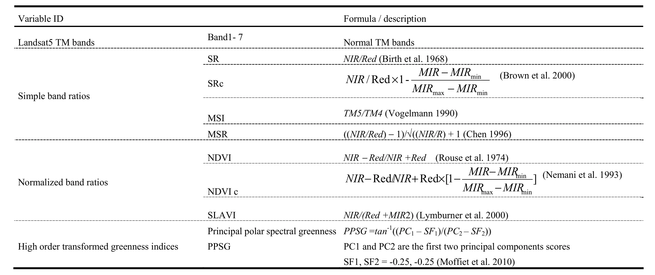
Table 3: Summary of Landsat TM derived variables

Statistical analysis

Most allometric equations for calculating field-based AGB are power models (Zianis et al. 2004), hence AGB and LiDAR derived variables are generally log transformed when developing regression models (Patenaude et al. 2005, Lu et al. 2012). In this study, the ground measured AGB, LiDAR derived variables and Landsat derived variables were log transformed. The BRNP andthe RRNP sites were analysed separately, and then again as a combined data set within a Multiple Linear Regression (MLR) framework. The statistical software (IBM SPSS 20) was employed to model average AGB using the best subsets regression procedure. Stepwise selection was performed to select independent variables to be included in final models. No independent variable was left in models with a partial F statistic with a significance level greater than 0.1 and included separately for each the study areas and the combined site. The variance inflation factors (VIF) greater than 10 was used to detect the multicollinearity of independent variables.

Regression diagnostics including R2, adjusted R2, relative root mean square error RMSE, and residual plots were used to select optimal models. Since the ground measured data of all sampling plots were used for model development, Predicted Residual Sum of Squares (PRESS) statistics was used as a form of cross validation. For the choice of the best model, one favours the model with the lowest PRESS.

Results

Results for each study area and the combined dataset (denoted‘combined’) were summarised for AGB estimates and the regression-based analysis (i.e. LiDAR, Landsat5 TM, and Li-DAR+Landsat5 TM estimates models).

LiDAR AGB estimates

The estimates models obtained using LiDAR derived variables of the two study areas and combined data are summarised in Table 4. The LiDAR derived four height related variables (i.e. ht_m, ht_med, ht_60th and ht_rmed), and fractional cover for canopy components were most significant for all predictive models of the three data sets investigated. These variables performed well with models significant at (p ＜0.0001). In terms of AGB estimates, the LiDAR based prediction model for the combined data set was the best, explaining 79% (0.79 adjusted R2) variation in measured values. Given the similar number of plots for the different plant communities, the RRNP AGB prediction models accounted for 31% more variation than for the BRNP. Fig. 3 shows the observed versus the predicted AGB by LiDAR, Landsat5 TM and LiDAR+ Landsat5 TM with the respective relative RMSE values in the BRNP and RRNP and combined. Fig. 3 indicates that the relative RMSE was greatest (18.4%) combined site data and BRNP site data, however, a large proportion of variation in ground estimated AGB was explained by LiDAR. Relative RMSE among the selected LiDAR based prediction models were lower for the RRNP at almost 12.5%.

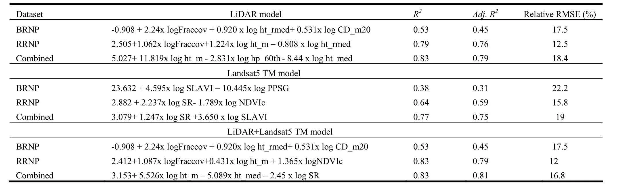
Table 4: Results for LiDAR, Landsat5 TM and LiDAR+Landsat5 TM based regression analysis of AGB estimates of the BRNP, the RRNP and combined data

Landsat5 TM estimates

Regression of individual Landsat5 TM model covariates resulted in the most acceptable model performance for individual sites rather than the combined sites, however, the overall performance was not as high as the LiDAR based AGB estimates models (Table 4 and Fig. 3). The best model fits were obtained from selection of the SR and SLAVI for the combined site data and these covariates explained 75% of variation in the ground measured AGB. For the estimation model of AGB in the RRNP, the SR, NDVI47, and SLAVI covariates were selected and the adjusted R2of overall predictive models was 0.59. It was found that the regression of Landsat5 TM model covariates for the BRNP sites performed poorly; SLAVI and PPSG were enabled to account for 31% of variation of response data. Fig. 3 shows that the lowest relative RMSE (15.8%) was found for the RRNP, and the least accurate results were produced for the BRNP (relative RMSE = 22%).

LiDAR+Landsat estimates

Table 4 shows the results of AGB estimate models by combining both LiDAR and Landsat5 TM derived variables. The RRNP and combined sites models using both sensors derived variables showed an enhancement of accuracy of prediction of AGB. The best model in terms of adjusted R2(0.81) was obtained from selection of both LiDAR and Landsat TM derived variables for the combined site data; respective relative RMSE (16.8%) wasgreater than the relative RMSE (12%) obtained for RRNP (see Fig. 3). However, Table 4 and Fig. 3 depicted that no improvement was evident for the AGB prediction model for the BRNP using a combination of variables of both sensors.

Overall, the combination of Landsat5 TM and LiDAR derived variables increased adjusted R2and decreased relative RMSE for the RRNP, and combined sites (Table 4 and Fig. 3), and the improvement for both cases was not much higher. For example, the RRNP integrated AGB prediction model improved adjusted R2from 0.76 to 0.79 and decreased relative RMSE by from 12.5 to 12 %. For all cases, the BRNP, the RRNP, and the combined AGB were free from multicollinearity (i.e. VIF ＜ 10), and all developed equations were parsimonious models that containing four or less than four independent variables.

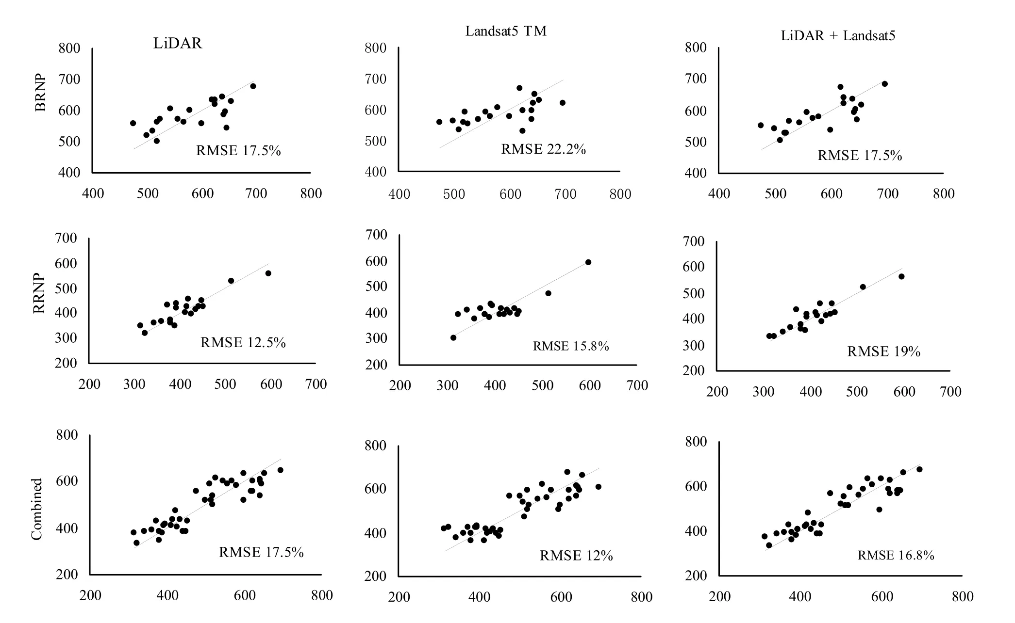
Fig. 3: Ground measured (X axis) versus predicted (Y axis) AGB for the models based on study area division: The solid lines show 1:1 relationship

Validation of the regression models prediction

Table 5 shows the cross-validation results of all candidate models. For the RRNP, and combined sites data, the cross-validation showed that integration of LiDAR and Landsat5 TM derived variables improved the prediction of AGB, revealing overall smaller PRESS statistics and standard deviation of PRESS residuals. The LiDAR derived variables based prediction models consistently gave satisfactory results for each data set as indicated by PRESS statistics. For each data set, the highest overall PRESS statistics and standard deviation of PRESS residuals were observed for Landsat5 TM derived variables based AGB prediction models.

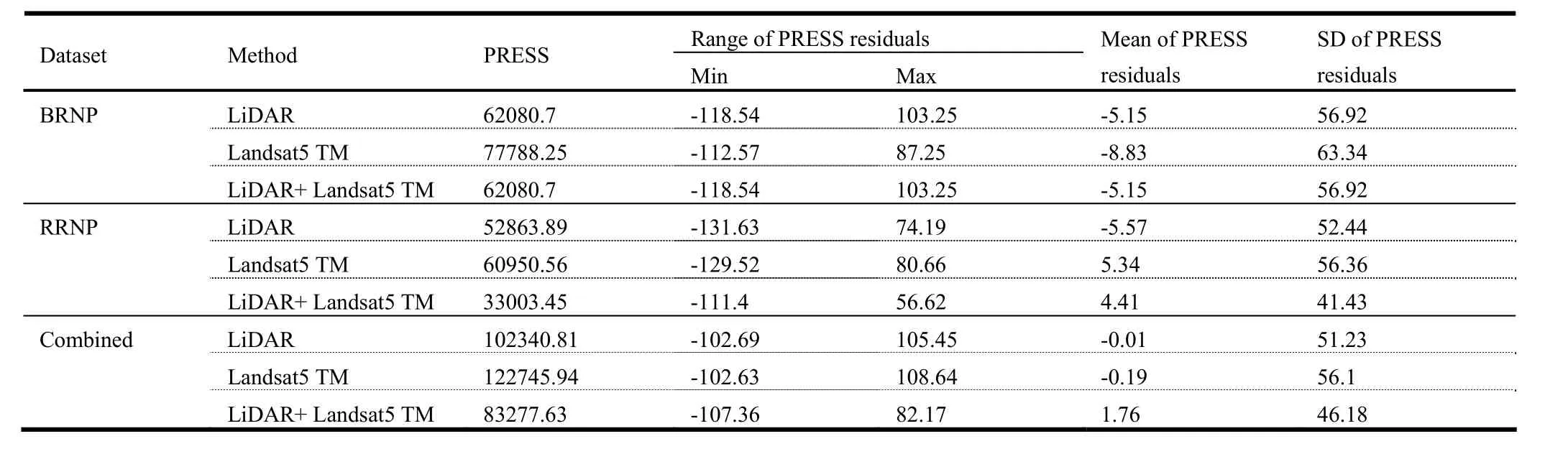
Table 5: PRESS statistics for predicting AGB for the BRNP, the RRNP and the combined sites data

In conclusion, the most accurate estimation results were obtained for LiDAR and Landsat5 TM derived variables integrated AGB prediction models for the RRNP, and this is followed by the combined sites data sets. The AGB estimation in the BRNP was less accurate, and the combination of LiDAR and Landsat5 TM covariates did not improve model performance.

Discussion

This study sought to improve the predicting capacity of plot-scale AGB estimation by combining LiDAR and Landsat5 TM derived variables for eucalypt dominated forest and subtropical rainforest. We anticipated that combining LiDAR derived variables with various Landsat5 TM derived vegetation indices would significantly improve accuracy of plot-scale AGB in the subtropical rainforest with complex terrain of the BRNP site. The findings revealed that fusing LiDAR and Landsat5 TM derived variables did not improve estimation of plot-scale AGB in the BRNP. However, estimation of plot-scale AGB by fusing LiDAR and Landsat5 TM enhanced the accuracy of prediction by improving adjusted R2and decreasing the RMSE for the open canopy RRNP, and combined sites data. This result conforms the expected findings for estimation of forest biomass (Popescu et al. 2004; Latifi et al. 2010) and other structural parameters of vegetation (Hudak et al. 2006; Tonolli et al. 2011). The most important and informative variables (e.g. tree height, LiDAR fractional cover, crown diameter) derived by LiDAR explained the largest proportion of variation in plot-scale AGB estimates among the three datasets. The accuracy of LiDAR based models improved the AGB estimation by 3% in the RRNP and 2% in the combined sites after integration of the Landsat5 TM derived variables. Although the accuracy of AGB prediction models for combined sites improved, its relative RMSE values were higher compared to all AGB prediction models developed by LiDAR, Landsat5 TM, and fusing both data. This is probably due to the increase in standard deviation of plot-scale ground measured AGB after combining individual sites data (Table 1).

This study fitted LiDAR derived variables in AGB estimation models that differed due to the number of variables and the structural component of vegetation between the study data sets. The results showed that that LiDAR derived overstorey height related variables tend to be those which have incorporated LiDAR based AGB estimation model for each data set investigated. The LiDAR metrics comprised of vertical and horizontal information about vegetation structure (i.e. tree height and canopy structure) are more likely to detect the structural components which are contained in the high biomass. For most forest types the bulk of AGB is located in tree stems, thus, inclusion of LiDAR derived height variables to estimate AGB results in more accurate predictions similar to findings by Bortolot et al. (2005) and Popescu (2007) who estimated AGB at individual tree scale, and Drake et al. (2002) and Drake et al. (2003) who estimated AGB at plot scale. LiDAR fractional cover was also instrumental in predicting significant amounts of plot-scale AGB in both plant communities. LiDAR fractional cover measures total photosynthetic and non-photosynthetic components of forest canopy (Weller et al. 2003), thus, it is possible to consider it as the second largest pool of accumulated AGB in vegetation. This is consistent with findings of previous studies (Li et al. 2008; Krasnow et al. 2009; Erdody et al. 2010) which have used similar information about canopy cover density and found this to be a key predictor of AGB. Estimating individual tree, or plot-scale AGB using LiDAR derived height variable is not new, however, this study is unique in its improvement of AGB estimation by incorporating a canopy component related variable such as LiDAR fractional cover. Ediriweera et al. (2014 accepted) revealed that inclusion of canopy attributes related to the LiDAR fractional cover with tree height for BA estimates prove that FPC is a key component for estimating basal area for Australian woody vegetation. Similarly Armston et al. (2009) found a strong allometric relationship between the FPC and stand basal area for Australian woody plant communities. In addition to that LiDAR fractional cover can improve the prediction ability of models as it lowers the vulnerability to errors created by variations in topography when compared to LiDAR derived tree height variable. The LiDAR estimated crown diameter moderately correlated with AGB estimates, however, the relationship was not as high as the height and Li-DAR fractional cover parameters in all sites. This finding is inconsistent with Popescu (2007) who showed that plot level tree crown diameter calculated from individual tree LiDAR measurements were particularly important in prediction of forest biomass in temperate forests. This is likely a failure to accurately delineate the tree crowns of broad leaf trees due to the complexity of the irregular shaped overlapped tree crowns, and the spatial organization of tree crowns within the canopy and inadequate LiDAR point density.

Landsat5 TM visible bands, and Landsat derived vegetation indices have potential to estimate AGB in forest areas. However, this study did not show any strong relationships for Landsat5 TM spectral signatures with ground measured AGB for either plant community. This finding is inconsistent with previous studies that have shown spectral signatures are highly related to biomass (Franklin 1986; Jakubauskas et al. 1997). This is probably due to the plots being located on different slopes and aspects in both study areas, thus, this seems to be a topographic effect which has not been effectively compensated for at the pixel and sub-pixel scale. Similarly, surface radiance is influenced by canopy height, however Landsat imagery is much more sensitive to the spectral properties of the surface materials than to their height (Hudak et al. 1999). Additionally, the utilised band ratios and vegetation indices showed varying degrees of success in estimating AGB of the testing data for both study areas. Vegetation indices are sensitive to internal factors (i.e canopy geometry, terrain factors, species composition), and external factors (i.e. sun elevation angle effect, atmospheric condition) that influence vegetation reflectance (Treitz et al. 1999) in topographically complex landscape. It was noted that specific leaf area vegetation index (SLAVI) (uses Landsat5 TM band 3, 4, and 7), and high order (6) dimensional set of Landsat5 TM derived principal polar spectral greenness (PPSG)only correlated with ground estimated AGB of the structurally complex BRNP. SLAVI was used to estimate the important ecophysiological characteristics of foliage, such as, specific leaf area which has a direct relationship with net photosynthesis (Reich et al. 1988; Reich et al. 1997) and above ground net primary productivity (Fassnacht et al. 1997). PPSG is assumed to be associated with spectral profile variations related to the projected aerial proportions of green photosynthetic material and substrate (Moffiet et al. 2010).

For the open forest in a dissected topography, the relationship between AGB and Landsat derived variables can be affected by background effect, and site factors such as topography and aspect. The relationship is sensitive to background, atmosphere, and bidirectional effects (Myneni et al. 1994). However, for the open canopy RRNP, NDVIc together with SR proved to be good predictors in estimating the AGB. The NDVIc is derived from multispectral remotely sensed data including red, NIR, and MIR bands (Nemani et al. 1993), and may be useful in accounting for understory effects in more open canopy forest and woodlands (Spanner et al. 1990; Nemani et al. 1993; Zheng et al. 2004). The RRNP study area was classified as eucalypts dominated open forest with mesic understorey (i.e. mixed grass, shrubs), which is more likely to be disturbed by tree felling and canopy dieback.

Sources of error and limitations

There are three main sources of error and limitations: (1) the field data collection and ABG estimation, (2) remotely sensed data processing, and (3) the influence of vegetation structure and topography.

Most re-growth stems were damaged by fire and heavily sprouted. Standing dead trees were found in most of the sample plots in the RRNP and were included in the dbh measurement, potentially influencing the accuracy of LiDAR information. Heurich et al. (2008) described that dead trees alter the distribution of laser readings, and can influence the accuracy of results. Additionally, dbh measurements for trees along the plot borderlines were problematic, particularly for groups of large trees in the BRNP. Due to the lack of allometric equations at the finest taxonomic resolution for the targeted plant communities, two general allometric equations were used. These equations adds potential error as the allometric relationships vary in response to climatic conditions, nutrient availability, genotype, age, and growth form of trees (Keith et al. 2000).

Topographically complex terrain results in topographic distortion, and vertical structure creates self-shadowing by overstorey trees thereby decreasing the amount of visible reflectance. It is likely the applied topographic correction method has not been effectively minimised for topographically induced illumination. Furthermore, Landsat5 TM with broad wavelength data are susceptible to saturation due to similar canopy structure and the impact of shadowing (Lu 2006).

The LiDAR sensor configuration and specification of LiDAR data acquisition have a strong influence on the accuracy of data due to the high flying altitude (2 km) reduced energy per pulse, and reduced strength of reflected signal. Due to dense foliage at the BRNP there were more LiDAR first returns from the overstorey, prohibiting high accuracy of LiDAR derived height information of lower strata. For instance Ediriweera et al. (2014 accepted) showed a significant error in estimation of mean and dominant canopy height (i.e. Adj. R20.40 and 0.61 for mean and dominant height respectively) using LiDAR metrics in the same study area. In contrast, the estimation of dominant and mean canopy height from LiDAR data achieved a high level of accuracy (error ＜3%) and explained over 80% of total variation in dominant height for open canopy eucalypts forest of the RRNP. Furthermore, laser pulses cannot discriminate small canopy holes from canopy attributes in dense foliage, consequently over estimating LiDAR fractional cover by measuring the collective mean of canopy components, and small holes in clumps of leaves. Large overstorey trees on sloping terrain extend their branches or whole tree crown down slope, thereby borderline trees influenced the extraction of LiDAR fractional cover that contained unnecessary information from outside the plot.

In conclusion, this study provides an analysis on the fusion of LiDAR and LiDAR and Landsat5 TM data for the estimation of AGB. Analysis indicated that LiDAR derived vegetation structural variables were able to describe significant amounts of variation on plot-scale AGB. Variables were most accurate for the open canopy RRNP, followed by the combined sites, and were least able to account for plot-scale AGB in the closed canopy BRNP. Several studies demonstrated that fusion of sensors have improved the accuracy of estimating AGB as well as timber volume, tree height, species identification, and fuel mapping (McCombs et al. 2003; Popescu et al. 2004, Mutlu et al. 2008; Erdody et al. 2010; Tonolli et al. 2011). This study reinforced that Landsat5 TM derived variables fused with LiDAR derived models increased overall performance for open canopy forest and combined sites by accounting for extra variation of field estimated plot-scale AGB. However, fusion LiDAR derived variables with Landsat5 TM derived spectral information data did not improve AGB estimation in closed canopy subtropical rainforest in topographically complex terrain. Both data missions employed a Leica ALS50-II LiDAR sensor and similar acquisition parameters (e.g. wave length, flight height, foot print size etc.). This study has demonstrated the potential for LiDAR datasets with similar acquisition parameters to be merged for regionwide estimates of AGB. Fusion LiDAR derived variables with Landsat5 TM derived spectral information data allows to improve accuracy of AGB prediction (3% for eucalypt forest and 2% combined sites) of hilly vegetation. However, this improvement was not significant when compared with data processing and computation cost.

Acknowledgements

The authors wish to acknowledge The Land and Property Management Authority, NSW for providing LiDAR data. This study was made possible by a scholarship from the Australian Government (International Postgraduate Research Scholarship-awarded in 2009) and a Southern Cross University Postgraduate Research Scholarship (SCUPRS in 2009). We especially thank Jonathan Parkyn, Thomas Watts, Agata Kula, Jim Yates, Susan Kerridge and Katherine Louise for fieldwork.

References

Armston JD, Denham RJ, Danaher TJ, Scarth PF, Moffiet TN. 2009. Prediction and validation of foliage projective cover from Landsat-5 TM and Landsat-7 ETM+ imagery. Journal of Applied Remote Sensing, 3: 1−28.

Birth GS, McVey G. 1968. Measuring the colour of growing turf with a reflectance spectrophotometer. Agronomy Journal, 60: 640−643.

Bortolot ZJ, Wynne RH. 2005. Estimating forest biomass using small footprint LiDAR data: An individual tree-based approach that incorporates training data. Isprs Journal of Photogrammetry and Remote Sensing, 59: 342−360.

Brown L, Chen JM, Leblanc SG, Cihlar J. 2000. A shortwave infrared modification to the simple ratio for LAI retrival in borel forests: and image and model analysis. Remote Sensing of Environment, 71: 16−25.

Bureau of Meterology. 2010. Bureau of Meteorology (ABN 92 637 533 532), Australia. Available at: http://www.bom.gov.au [accessed on 2 August 2012].

Chambers JQ, dos Santos J, Ribeiro RJ, Higuchi N. 2001. Tree damage, allometric relationships, and above-ground net primary production in central Amazon forest. Forest Ecology and Management, 152: 73−84.

Chave JH, Andalo C, Brown S,Cairns MA,Chabbers JQ, Eamus D, Folster H,Fromard F,Higuchi N,Kira T,Lescure JP,Nelson BW,Ogawa H, Puig H, Riera B,Yamakura T. 2005. Tree allometry and improved estimation of carbon stocks and balance in tropical forests. Oecologia, 145: 87−99.

Chen JM. 1996. Evaluation for vegetation indices and modified simple ration for boreal application Canadian Journal of Remote Sensing, 22: 229−242.

Drake JB, Dubayah RO, Knox RG, Clark DB, Blair JB. 2002. Sensitivity of large-footprint LiDAR to canopy structure and biomass in a neotropical rainforest. Remote Sensing of Environment, 81: 378−392.

Drake JB, Knox RG, Dubayah RO, Clark DB, Condit R, Blair JB, Hofton M. 2003. Above-ground biomass estimation in closed canopy Neotropical forests using lidar remote sensing: factors affecting the generality of relationships. Global Ecology and Biogeography, 12: 147−159.

Ediriweera S, Pathirana S, Danaher T, Nichols D. 2014 (accepted). LiDAR remote sensing of structural properties of subtropical rainforest and eucalypt forest in complex terrain in North-eastern Australia. Journal of Tropical Forest Science.

Erdody TL, Moskal LM. 2010. Fusion of LiDAR and imagery for estimating forest canopy fuels. Remote Sensing of Environment, 114: 725−737.

Fassnacht KS, Gower ST. 1997. Interrelationships between the edaphic and stand characteristics, leaf area index and above ground next primary productivity of upland forest ecosystems in north central Wisconsin. Canadian Journal of Forestry, 27: 1058−1067.

Flood N, Danaher T, Gill T, Gillingham S. 2013. An Operational Scheme for Deriving Standardised Surface Reflectance from Landsat TM/ETM+ and SPOT HRG Imagery for Eastern Australia. Remote Sensing, 5: 83−109.

Florence RG. 1996 Ecology and Silviculture of Eucalypt Forests. CSIRO Australia.

Foody GM, Boyd DS, Cutler MEJ. 2003. Predictive relations of tropical forest biomass from Landsat TM data and their transferability between regions. Remote Sensing of Environment, 85: 463−474.

Foody GM, Cutler ME, McMorrow J, Pelz D, Tangki H, Boyd DS, Douglas I. 2001. Mapping the biomass of Bornean tropical rain forest from remotely sensed data. Global Ecology and Biogeography, 10: 379−387.

Franklin J. 1986. Thematic mapper analysis of coniferous forest structure and composition. International Journal of Remote Sensing, 7: 1287−1301.

Heurich M, Thoma F. 2008. Estimation of forestry stand parameters using laser scanning data in temperate, structurally rich natural European beech (Fagus sylvatica) and Norway spruce (Picea abies) forests. Forestry, 81: 645−661.

Hudak AT, Crookston NL, Evans JS, Falkowski MJ, Smith AMS, Gessler PE, Morgan P. 2006. Regression modelling and mapping of coniferous forest basal area and tree density from discrete- return LiDAR and multispectral satellite data. Canadian Journal of Remote Sensing, 32: 126−138.

Hudak AT, Lefsky MA, Cohen WB. 2001: Integration of lidar and Landsat ETM data. In: Hofton, M.A. (ed.), The international archives of the Photogrammetry, Remote Sensing and Spatial Information Science. Volume XXXIV, Part 3/W4, Commission III, Annapolis MD, 22–24 October, pp.95–104

Jakubauskas ME, Price KP. 1997. Empirical relationaship between structural and spectral factors of Yellowstone Lodgepole Pine Forests. Photogrammetric Engineering & Remote Sensing, 63: 1375−1381.

Jensen JLR, Humes SK, Vierling LA, Hudak AT. 2008. Discrete return LiDAR based prediction of leaf area index in two conifer forests. Remote Sensing of Environment, 112: 3947−3957.

Krasnow K, Schoennagel T, Veblen TT. 2009. Forest fuel mapping and evaluation of LANDFIRE fuel maps in Boulder country, Colorado, USA. Forest Ecology and Management, 257: 1603−1612.

Latifi H, Nothdurft A, Koch B. 2010. Non-parametric prediction and mapping of standing timber volum and biomass in a temperature forest. Application of multiple optical/LiDAR-derived predictors. Forestry, 83: 395−407.

Li Y, Andersen HE, McGaughey R. 2008. A comparison of statistical methods for estimating forest biomass from light detection and ranging data. Western Journal of Applied Forestry, 23: 223−231.

Lovell JL, Jupp DLB, Culvenor DS, Coops NC. 2003. Using airborne and ground-based ranging lidar to measure canopy structure in Australian forests. Canadian Journal of Remote Sensing, 29: 607−622.

Lu D. 2006. The potential and challenge of remote sensing based biomass estimation. International Journal of Remote Sensing, 27: 1297−1328.

Lu D, Batistella M. 2005. Exploring TM image texture and its relationships with biomass estimation in Rondonia, Brazilian Amazon. Acta Amazonica, 35: 261−268.

Lu D, Chen Q, Wang G, Moran E, Batistella M, Zhang M, Vaglio LG, Saah D. 2012. Aboveground Forest Biomass Estimation with Landsat and LiDAR Data and Uncertainty Analysis of the Estimates. International Journal of Forestry Research, 2012: 16.

Lymburner L, Beggs PJ, Jacobson CR. 2000. Estimation of canopy-average surface-specific leaf area using Landsat TM data. Photogrammetric Engineering and Remote Sensing, 66: 183−191.

Markham BL, Helder DL. 2012. Forty-year calibrated record of earth-reflected radiance from Landsat: A review. Remote Sensing of Environment, 122 30−40.

McCombs JW, Roberts SD, Evans DL. 2003. Influence of fusing LiDAR and multispectral imagery on remotely sensed estimates of stand density and mean tree height in managed Loblolly pine plantation. Forest Science, 49: 457−466.

Moffiet T, Armston JD, Mengersen K. 2010. Motivation, development and validation of a new spectral greenness index: A spectral dimension related to foliage projective cover. Isprs Journal of Photogrammetry and Remote Sensing, 65: 26−41.

Mutlu M, Popescu SC, Stripling C, Spencer T. 2008. Mapping surface fuel models using lidar and multispectral data fusion for fire behavior. Remote Sensing of Environment, 112: 274−285.

Myneni RB, Williams DL. 1994. On the Relationship between FAPAR and NDVI. Remote Sensing of Environment, 49: 200−211.

Nemani R, Pierce L, Running S, Band L. 1993. Forest ecosystem processes at the watershed scale: sensitivity to remotely-sensed Leaf Area Index estimates. International Journal of Remote Sensing, 14: 2519–2534.

Patenaude G, Milne R, Dawson TP. 2005. Synthesis of remote sensing approaches for forest carbon estimation: reporting to the Kyoto Protocol. Environmental Science and Policy, 8: 161−178.

Popescu SC. 2007. Estimating biomass of individual pine trees using airborne LiDAR. Biomass and Bioenergy, 31: 646−655.

Popescu SC, Wynne RH, Nelson RF. 2003. Measuring individual tree crown diameter with LiDAR and assessing its influence on estimating forest volume and biomass. Canadian Journal of Remote Sensing, 29: 564−577. Popescu SC,Wynne RH, Scrivani JA. 2004. Fusion of Small-Footprint Lidar and Multispectral Data to Estimate Plot- Level Volume and Biomass in Deciduous and Pine Forests in Virginia, USA. Forest Science, 50: 551−565.

Reich PB, Walters MB, Ellsworth DS. 1997. From tropic to tundra: Global convergence in plant functioning. In: Proceeding of the National Academy of Sciences, pp. 13730−13734, USA.

Reich PB, Walters MB, Ellsworth DS, Vose JM, Volin JC, Gresham C, Bowman WD. 1988. Relationships of leaf dark respiration and leaf area index to specific leaf area and leaf life -span: A test across biomes and functional group Oecologia, 114: 471−482.

Riggins JJ, Tullis JA, Stephen FM. 2009. Per-segment Aboveground Forest Biomass Estimation Using LIDAR-Derived Height Percentile Statistics. Gioscience & Remote Sensing, 46: 232−248.

Rouse JW, Haas RH, Schell JA, Deering DW. 1974. Monitoring vegetation systems in the Great Plains with ERTS. In: Third Earth Resources Technology Satellite-1 Symposium. NASA SP-351, Greenbelt, Md., Woshington DC. pp. 301−317.

Roy PS, Ravan SA. 1996. Biomass estimation using satellite remote sensing data-an investigation on possible approaches for natural forest. Journal of Biosciencce, 21: 535−561. Smith RGB, Nichols JD, Vanclay JK. 2005. Dynamics of tree diversity in undisturbed and logged subtropcal rainforest in Australia. Biodiversity and Conservation, 14: 2447−2463.

Spanner MA, Pierce LL, Peterson DL, Running SW. 1990. Remote sensing of temperate coniferous forest leaf area index The influence of canopy closure, understory vegetation and background reflectance. International Journal of Remote Sensing, 11: 95–111.

Specht A,West PW. 2003. Estimation of biomass and sequestered carbon on farm forest plantations in northern New South Wales Australia. Biomass Bioenergy, 25: 363−379.

Specht RL, Specht A. 1999 Australian plant communities: dynamics of structure, growth and biodiversity.Oxford University Press.

Tonolli S, Dalponte M, Neteler M, Rodeghiero M,Vescovo L, Gianelle D. 2011. Fusion of airborne LiDAR and satellite multispectral data for the estimation of timber volume in the Southern Alps. Remote Sensing of Environment, 115: 2486−2498.

Treitz PM, Howarth PJ. 1999. Hyperspectral remote sensing for estimating biophysical parameters of forest ecosystems. Progress in Physical Geography, 23: 359−390.

Vermote FE,Tanre D, Deuze JL, Herman M, Morcrette JJ. 1997. Second Simulation of the Satellite Signal in the Solar Spectrum, 6S: Overview. Ieee Transactions on Geoscience and Remote Sensing, 35: 675−686.

Vogelmann JE. 1990. Comparison between two vegetation indices for measuring different types of forest damage in the northeastern United States. International Journal of Remote Sensing, 11: 2281−2297.

Weller D, Denham R, Witte C, Mackie C, Smith D. 2003. Assessment and monitoring of foliage projected cover and canopy height across native vegetation in Queensland, Australia, using laser profiler data. Canadian Journal of Remote Sensing, 29: 578−591.

Westman WE, Rogers RW. 1977. Biomass and structure of a subtropical eucalypt forest, North Stradbroke Island. Australian Journal of Botany, 25: 171−19.

Zheng D, Rademacher J, Chen J, Crow T, Bresee M, Le Moine J, Ryu SR. 2004. Estimating aboveground biomass using Landsat 7 ETM+ data across a managed landscape in northern Wisconsin, USA. Remote Sensing of Environment, 93: 402−411.

Zianis D, Mencuccini M. 2004. On simplifying allometric analyses of forest

biomass. Forest Ecology and Management, 187: 311−332.

DOI 10.1007/s11676-014-0485-7

Project funding: This study was made possible by a scholarship from the Australian Government (International Postgraduate Research Scholarship-awarded in 2009) and a Southern Cross University Postgraduate Research Scholarship (SCUPRS in 2009)

The online version is available at http://www.springerlink.com

Sisira Ediriweera (), Sumith Pathirana , Doland Nichols

School of Environment, Science and Engineering, Southern Cross University, Lismore, NSW 2480 Australia

Tim Danaher

Office of Environment and Heritage, Alstonville, NSW 2477 Australia

*Correspondence details: Address: Faculty of Science and Technology, Uva Wellassa University, Badulla, Sri Lanka.

Tel. +94553559113; Fax: + 94 552226472

Email: sisira@uwu.ac.lk

Corresponding editor: Chai Ruihai