Notes on well-posedness for the b-family equation
2014-09-06ZhuMin
Zhu Min
(Department of Mathematics, Southeast University, Nanjing 211189, China)(Department of Mathematics, Nanjing Forestry University, Nanjing 210036, China)
Notes on well-posedness for the b-family equation
Zhu Min
(Department of Mathematics, Southeast University, Nanjing 211189, China)(Department of Mathematics, Nanjing Forestry University, Nanjing 210036, China)

b-family equation; Besov space; local well-posedness
We consider the b-family shallow water equation[1-4], namely,
mt-Aux+umx+buxm+γuxxx=0t>0,x∈R
(1)
with initial datam(0,x)=u0(x)-α2u0,xx, whereu(t,x) stands for the horizontal velocity of the fluid,u→0 asx→∞;Ais a nonnegative parameter related to the critical shallow water speed and the parameter is a constant. The real dimensionless constantbis a parameter, which provides the competition, or balance, in fluid convection between nonlinear steepening and amplification due to stretching, it is also the number of covariant dimensions associated with the momentum densitym. With the momentum densitym=u-uxx, Eq.(1) can be rewritten as
ut-α2utxx-Aux+(b+1)uux+γuxxx=α2(buxuxx+uuxxx)
(2)
Eq.(2) can be regarded as a model of water waves by using asymptotic expansions directly in the Hamiltonian for Euler’s equation in the shallow water regime[5-6]. Eq.(2) is the Korteweg-de Vries (KdV) equation when the parametersα=0 andb=2 and the Camassa-Holm (CH) equation when the pararmeteb=2[7]. Eq.(2) is also referred to as the Dullin-Gottwald-Holm (DGH) equation[5,7]whenb=2 andγ≠0 and the Degasperis-Procesi (DP) equation whenb=3[5-6,8-10]. The KdV equation, the CH equation and the DP equation[8]are the only three integrable equations in the b-family equation.
The problem of finding the largest spacesEfor which Eq.(1) with initial data inEis well-posedness in the mean of Hadamard has attracted a lot of attention recently. Before going further into details, let us define what we mean by local well-posedness in the mean of Hadamard.
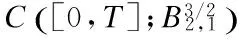
Definition 1 LetEbe a Banach space. Eq.(1) is said to be locally well-posedness inEin the mean of Hadamard if for anyu0∈E, there exists a neighborhoodVofu0andT>0 such that for anyv0∈V, Eq.(1) has a unique solutionv∈C([0,T];E) with initial datumv0, and the mapv0→vis continuous fromVintoC([0,T];E).
(3)
If we denoteP(D) as the Fourier integral operator with the Fourier multiplier -iξ(1+ξ2)-1, then Eq.(3) becomes
(4)

1 Preliminaries
In this section, we will recall some facts on the Littlewood-Paley decomposition, the nonhomogeneous Besov spaces and some of their useful properties. The transport equation theory will be used in the following section.
Proposition 1[11](Littlewood-Paley decomposition) There exists a couple of smooth functions (χ,φ) valued in [0,1], such thatχis supported in the ballBφis supported in the ringCφ(2-qξ)=1, suppφ(2-q·)∩suppφ(2-q′·)(·)∩suppφ(2-q·)=φ(q≥1).
Then for allu∈S′, we can define the nonhomogeneous dyadic blocks as follows. LethF-1φandF-1χ. Then the dyadic operatorsΔqandSqcan be defined as follows:
Δquφ(2-qD)u=2qn∫Rnh(2qy)u(x-y)dyq≥0
Squ
Δ-1uS0u,Δqu0q≤-2
Hence,
where the right-hand side is called the nonhomogeneous Littlewood-Paley decomposition ofu.

Inthefollowingproposition,welistsomeimportantpropertiesoftheBesovspace.

Lemma 1[13-14](a priori estimates in Besov space)
(5)
Moreover, there exists a constantConly depending ons,pandr, such that the following statements hold:

and


In order to apply the contraction argument to prove the analytic regularity of the Cauchy problem (3), we need a suitable scale of Banach spaces which we will describe below.
For anys>0, we set

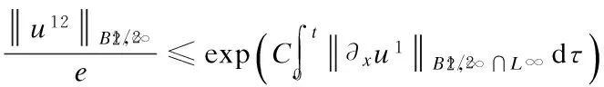
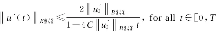
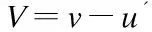
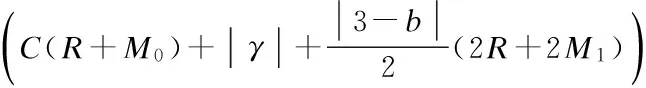
Lemma 5[15]There is a constantc>0 such that for any 0 The following lemma comes from Ref.[6]. (6) LetT,RandCbe the positive constants. Assume thatFsatisfies the following conditions: Moreover, the solution depends continuously on the initial data; i.e., the mapping is continuous. The first step is to prove the existence of the solution. Uniqueness is a corollary of the following result. (7) then, denotingL(z)=zlog(e+z), the following inequality holds true fort∈[0,T*], (8) Proof We know thatu12solves the following linear transport equation: (9) where By virtue of Lemma 1, the following inequality holds true: (10) UsingProposition2andthankstothefollowingtwoproperties: Wereadilyobtain (11) and (12) Pluggingtheaboveinequalitiesin(10)andusingthelogarithmicinterpolation(Proposition2 (2)),weinferthat (13) (1-logW(τ))dτ (14) provided thatw(t)≤1 on [0,t]. Combining hypothesis (7) with a Gronwall’s inequality yields which is the desired result. is continuous. The main ingredients for proving Lemma 9 are Proposition 2 and a continuity result Lemma 1 for linear transport equations. Now combining the above uniform bounds with Proposition 3, we infer that Note thatv(n)solves the following linear transport equation: where f(n)= -(∂xun)2+bP(D)(un∂xun)+ Following Kato[17], we decomposev(n)intov(n)=z(n)+w(n)with and Therefore, the product laws in Besov spaces yield (15) Letε>0. Combining the above result of convergence with estimate (14), one concludes that for large enoughn∈N, for some constantCM,T,|γ|,b,Adepending only onM,T,γ,A,b. We obtain the desired result of this lemma. In this section, we shall establish the analyticity result. We restate the Cauchy problem in a more convenient form. Note that (3) is equivalent to the following form: (16) Differentiating with respect tox, we obtain that (17) Letv=ux. Then the problem can be written as a system foruandv: (18) (19) This can be written as the abstract form of the Cauchy problem. We shall establish the following analyticity result. Theorem 2 Letu0be a real analytic function on R. There existsε>0 and unique solutionuof the Cauchy problem (18) that is analytic on (-ε,ε). In order to prove 1), for 0 And hence condition 1) holds. Since Using Lemmas 4 and 5, we obtain the following estimates: and This implies that the condition (2) also holds. Hence, the proof of Theorem 2 is complete. [1]Constantin A, Ivanov R. On the integrable two-component Camassa-Holm shallow water system [J].PhysLettA, 2008, 372(48): 7129-7132. [2]Ivanov R. Two-component integrable systems modelling shallow water waves: the constant vorticity case [J].WaveMotion, 2009, 46(6): 389-396. [3]Olver P, Rosenau P. Tri-Hamiltonian duality between solitons and solitary wave solutions having compact support [J].PhysRevE, 1996, 53(2): 1900-1906. [4]Zhu M, Xu J X. On the wave-breaking phenomena for the periodic two-component Dullin-Gottwald-Holm system [J].JMathAnalAppl, 2012, 391(2): 415-428. [5]Dullin R, Gottwald G, Holm D. An integrable shallow water equation with linear and nonlinear dispersion [J].PhysRevLett, 2001, 87(19): 4501-4504. [6]Holm D D, Staley M F. Wave structure and nonlinear balances in a family of evolutionary PDEs [J].SIAMJApplDynSyst, 2003, 2(3): 323-380. [7]Camassa R, Holm D D. An integrable shallow water equation with peaked solitons [J].PhysRevLett, 1993, 71(11): 1661-1664. [8]Degasperis A, Holm D D, Hone A N W. A new integral equation with peakon solutions [J].TheoretMathPhys, 2002, 13(2): 1463-1474. [9]Dullin R, Gottwald G, Holm D, et al. Camassa-Holm, Korteweg-de Vries-5 and other asymptotically equivalent equations for shallow water waves [J].FluidDynRes, 2003, 33(1/2): 73-79. [10]Ivanov R. Water waves and integrability [J].PhilosTransRoySoc, 2007, 365(1858): 2267-2280. [11]Chemin J Y, Lerner N. Flot de champs de vecteurs non lipschitziens et equations de Vavier-Stokes[J].JDifferentialEquations, 1995, 121(2): 314-328. [12]Danchin R. A note on well-posedness for Camassa-Holm equation [J].JDifferentialEquations, 2003, 192(2): 429-444. [13]Danchin R. A few remarks on the Camassa-Holm equation [J].DifferentialandIntegralEquations, 2001, 14(8): 953-988. [14]Danchin R. A note on well-posedness for Camassa-Holm equation[J].JDifferentialEquations, 2003, 192(2): 429-444. [15]Himonas A A, Misiolek G. Analyticity of the Cauchy problem for an integrable evolution equation [J].MathAnn, 2003, 327(3): 575-584. [16]Baouendi M S, Goulaouic C. Sharp estimates for analytic pseudodifferential operators and application to the Cauchy problems [J].JDifferentialEquations, 1983, 48(2): 241-268. [17]Kato T. Quasi-linear equations of evolution, with applications to partial differential equations [C]//LectureNotesinMathematics. Berlin: Springer, 1975, 448: 25-70. b-family方程局部适定性注记 朱 敏 (东南大学数学系,南京 211189) (南京林业大学数学系,南京 210036) b-family方程;Besov空间;局部适定性 O175 The Natural Science Foundation of Higher Education Institutions of Jiangsu Province (No.13KJB110012). :Zhu Min. Notes on well-posedness for the b-family equation[J].Journal of Southeast University (English Edition),2014,30(1):128-134. 10.3969/j.issn.1003-7985.2014.01.024 10.3969/j.issn.1003-7985.2014.01.024 Received 2012-12-22. Biography:Zhu Min (1981—), female, doctor, zhumin@njfu.edu.cn.


2 Local Well-Posedness in


3 Analyticity of Solution


猜你喜欢
杂志排行

Journal of Southeast University(English Edition)的其它文章
- Speech emotion recognitionusing semi-supervised discriminant analysis
- Shape retrieval using multi-level included anglefunctions-based Fourier descriptor
- Performance analysis of ammonia-water absorption/compression combined refrigeration cycle
- Optimization of cross-coupling reaction for synthesis of antitumor drug vismodegib
- Flexural behaviors of FRP strengthened corroded RC beams
- Icon memory research under different time pressures and icon quantities based on event-related potential