A Novel Semi-Analytic Meshless Method for Solving Twoand Three-Dimensional Elliptic Equations of General Form with Variable Coefficients in Irregular Domains
2014-04-16YuReutskiy
S.Yu.Reutskiy
1 Introduction
In this paper we present a novel semi-analytic meshless method for numerical solv
ing 2D and 3D elliptic PDEs of the general form:
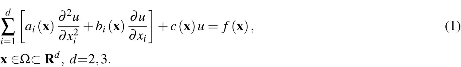
Here the coefficientsare smooth enough functions,ai(x)provide the elliptic type of the PDE andis the domain of a general form.
We supplement(1)with the boundary condition:

where the boundary operatorwill be de fined separately in each case.
Such problems often arise in many branches of applied science.Thus,during the last decades many numerical techniques have been developed in this field.In particular,there has been an increasing interest in the idea of meshless or mesh-free numerical methods for solving partial differential equations(PDEs).These methods are nowadays the main stream in numerical computations,as strongly advocated by many researchers,for example,Zhu,Zhang and Atluri(1998a,b);Atluri and Zhu(1998a,b);Atluri,Liu,and Kuo(2009);Atluri and Shen(2002);Cho,Golberg,Muleshkov,and Li(2004);Jin(2004);Li,Lu,Huang and Cheng(2007);Liu(2007a,b);Tsai,Lin,Young and Atluri(2007);Young,Chen,Chen and Kao(2007)In[Tsai,Liu and Yeih(2010)]the fictitious time integration method(FTIM)previously developed by Liu and Atluri(2008a,b)is combined with the method of fundamental solutions and the Chebyshev polynomials to solve Poisson-type PDEs.In this connection we should also note the MLPG method reviewed by Sladek,Stanak,Han,Sladek and Atluri(2013)which is a fundamental base for the derivation of many meshless formulations.In the last decade,a broad community of researchers and scientists contributed to the development and implementation of the MLPG method in a wide range of scientific disciplines.
For the past two decades radial basis functions(RBFs)have played an important role in the development of meshless methods for solving PDEs:Kansa(1990a,b);Kansa and Hon(2000);Golberg and Chen(1997);Golberg,Chen and Bowman(1999);Power(2002);Larsson and Fornberg(2003);Li,Cheng and Chen(2003);Cheng and Cabral(2005).A significant place among these techniques is taken up by methods based on the use of particular solutions.
In this approach,RBFs have been used to approximate the particular solution corresponding to the givenfand the original inhomogeneous PDE has been converted into a homogeneous one,so that one can apply the MFS or other boundary methods developed by Golberg and Chen(1997);Golberg,Chen and Bowman(1999);Cheng(2000).This is the so-called two-stage scheme:Note that similar technique has been developed with the use of the Chebishev polynomials instead of the RBFs by Cheng(2000);Golberg,Muleshkov,Chen and Cheng(2003);Cheng,Ahtes,and Ortner(1994);Tsai(2008)and for the spline approximation offby Tsai,Cheng and Chen(2009).
The scheme which combines the MFS and RBFs approximation has been proposed for further improvement of the MFS for solving PDEs with variable coefficients.This is the so-called one-stage scheme or the MFS-MPS technique[Chen,Fan and Monroe(2008)]:Recently this technique has been transformed into the method of approximate particular solutions(MAPS)Chen,Fan and Wen(2010,2011).Applying it to the problem

The information on the recent development of the MFS can be found in[Fu,Chen,and Yang(2009,2013)]and in proceedings cited in Chen,Fan and Monroe(2008).Similar to Kansa’s approach the unknownspiare determined by the collocation at the inner points of the solution domain and by the collocation of the boundary conditions.The collocation at the inner points is performed for equation(8)and this technique utilizes expansion(6)to approximate the boundary condition(4).More detailed information on the method can be found in the original papers cited above.In[Li,Chen and Tsai(2012)]the MAPS is applied for solving the Cauchy problems of elliptic partial differential equations with variable coefficients.The recent developments and advances on the RBF technique can be found in[Huang(2007);Cheng(2012);Chen,Hon and Schaback(2014)].
In Reutskiy(2012,2013)the semi-analytic meshless method(SAMM)was proposed for solving the equation

Similar to MPS it uses the particular solutions corresponding to the RBFs placed in the right hand side of the PDE.Let the basis functionsϕm(x)be such thatFcan be approximated by the linear combination

It is assumed that there exist analytic solutionscorresponding to the basis functionsϕm(x),which satisfy the equations:and the homogeneous boundary condition.The exact solution
is considered as an approximate solution of the boundary value problem(9),(2).We name this method as the indirect scheme of SAMM.See Reutskiy(2012,2013)for more detailed information.
In this paper we present the direct scheme of the SAMM which is as follows.Letug(x)be a smooth enough function in Ω and let it satisfy the boundary condition

Letϕm(x)be system of basis functions on Ω which satisfy the homogeneous boundary condition:

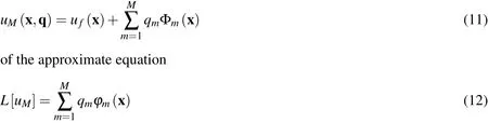
We seek an approximate solution in the form:

(cf.(11))which satisfies the boundary condition(2)with any choice of the free parametersq1,...,qM.The unknown free parameters are determined by substituting(15)in(1)and collocation at the inner points of Ω.Thus,the new direct scheme of the SAMM saves the key idea of the previous indirect scheme:the approximation of the boundary conditions and approximation of the PDE inside domain are algorithmically divided.
The outline of this paper is as follows.The main algorithm of the method is described in Section 2.The numerical implementation of the algorithm for 2D and 3D problems is presented in Section 3.In particular,the method is applied to the PDE with variable coefficients in the main operator part.Finally,in Section 4,we give a short conclusion.
2 Main algorithm
Throughout the paper we use the following RBFs:
1)the conical radial basis functions
Using these RBFs,we denote

and de fine the basis functions as:

where the centersξmare placed inside the solution domain Ω andthe correcting functions ωm(x)are chosen to satisfy the boundary condition(14):

It is important to note that contrary to the indirect SAMM here the functionsandug(x)should not necessarily satisfy any equation inside the solution domain.Thus,to approximate the correcting functionsωm(x)and the functionwe can use any complete in Ω system of functions.
When we have the basis functionswe substitutein the initial equation(1).Then we find the coefficientsby collocation inside the solution domain.be collocation points distributed inside the solution domain Ω.As a result of the collocation,we get the system ofNlinear equations for

All the terms in(18)can be obtained in the analytic form using the explicit expressions forφm,ωmandug.We take the number of the collocation pointsNto be approximately 2M.As a result we obtain an overdetermined linear system which can be solved by the standard least squares procedure.After determiningwe get the approximate solutionuM(x,q)(15).
3 Numerical results
3.1 Two-dimensional problems
The functions

form a complete orthogonal system inand
form a complete orthogonal system in the square
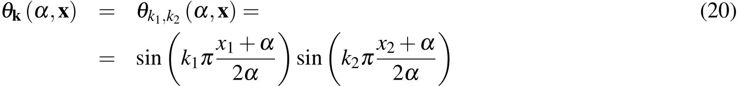
Choosingαlarge enough to satisfy Ω⊂Ωα,we look for the correcting functions in the form:

The number of terms in the sum(21)and the number of the unknownspm,kis:KI=the number of the different trigonometric products

withk1+k2≤I.We use 15≤I≤24 and so 120≤KI≤300 in all the calculations presented in this section.Using the collocation procedure,we get the linear system:

In the same way we look for the functionugin the form:

and obtain the system

We take the number of the collocation pointsK1to be approximately 2KI.
To validate the numerical accuracy,we calculate the following root mean square(RMS)errorserms:
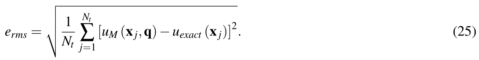
The same RMS errorex,rmsis used for thexderivative of the solution.We useNt=1000 test points randomly distributed inside Ω.We also use the maximum absolute erroremaxto estimate the accuracy of the calculations.
Example 1.Consider the equation:
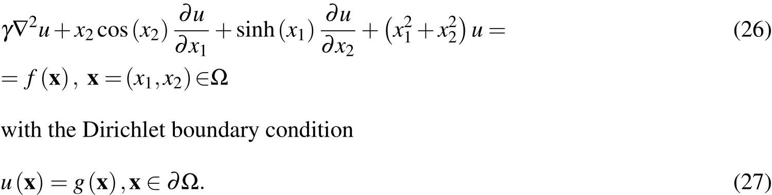
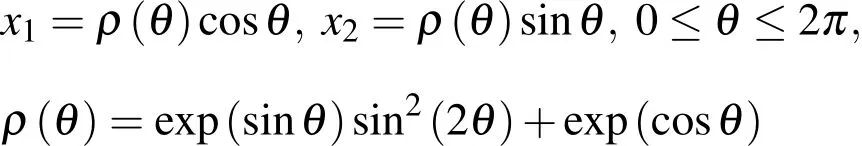
The computational domain is a star-shape domain with the boundary de fined by the parametric equation:

where(ρ,θ)are the polar coordinates.The domain is shown in Fig.1.
The functionsf(x)andg(x)correspond to the exact solution
一杭趴在雪萤的胸前安静了。雪萤感到大腿上有一点湿。但她没有多想,右手伸向提包的拉链,以咳嗽声掩盖拉链轻微的响声,迅速拿出匕首,高高地举起。

The data placed in Table 1 show the maximum absolute errorsemaxand the RMS errors in the solution of(26),(27)using MQ RBFs as the basis functions.The same problem was considered by Chen,Fan and Wen(2011)using the method of particular solutions(MPS)and Kansa’s method.The better results in solution this BVP presented there are:ni=317,nb=150:erms=8.95×10⁻⁶,ex,rms=9.98×10⁻⁵-for the MPS anderms=6.64×10⁻⁷,ex,rms=1.21×10⁻³-for Kansa’s method.
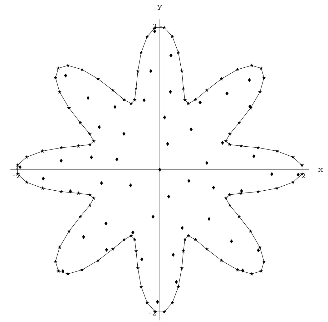
Figure 1:Example 1.The star-shape domain.The collocation points xnfor approximation PDE are shown inside the domain and the collocation points yifor approximation the correcting functions ωmare placed on the boundary ∂ Ω.
It should be noted that determination of the optimal shape parametercoptis a difficult problem in the framework of the presented method.As it is shown in Fig.2,the curveerms(c)is not monotonic and has many local minimums.The data placed in Table 1 correspond to some of these local minimums.However,there are quite enough other values of 0<c<1 which correspond to very close values oferms.For example,forM=50:erms(0.097)=1.054×10⁻⁷,erms(0.204)=1.050×10⁻⁷,erms(0.228)=1.040×10⁻⁷.

Figure 2:Example 1.The star-shape domain.The RMS errors ermsas functions of the MQ shape parameter c with different M.
The bottom part of the table contains the data corresponding to the small parameterγ=0.001 as a multiplier before the Laplace operator.Such problems are more difficult for numerical simulation.The numerical experiments carried out show that the proposed meshless scheme is very stable for a large range of values ofγ.In addition no fictitious source points are required in this version of the direct scheme of the SAMM.The data obtained by using the RBFsandas the basis functions are placed in Table 2.They show that the use of RBFsprovides approximately the same accuracy of the calculation as MQ.But they do not require any efforts for optimization.
Example 2Consider the following Poisson equation

The exact solution is given byThe data obtained by using the RBFsas the basis functions are placed in Table 3.This problem was also studied by Wei,Chen and Fu(2013)using the singular boundary method.The better result obtained there iserms~10-5.
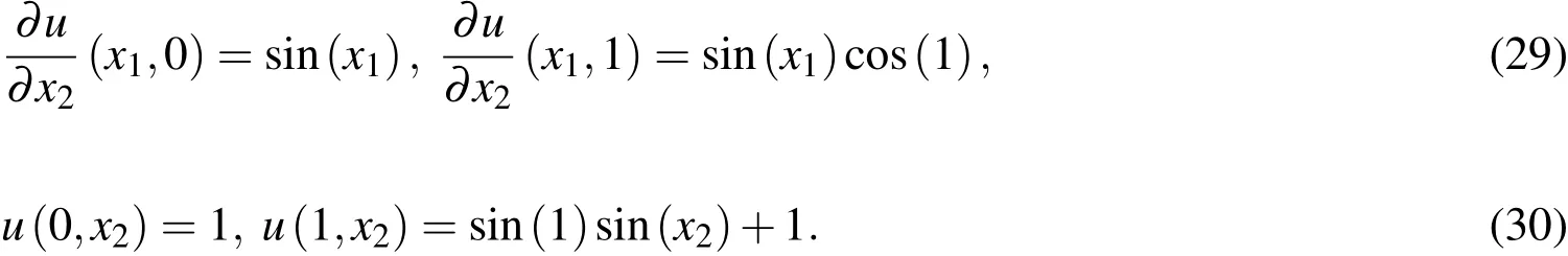
Example 3.Consider the equation with variable coefficients in the main operator part:
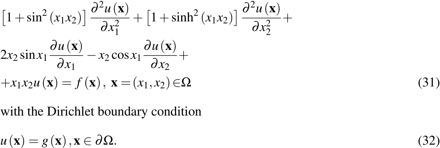

Table 1:Example 1.The maximum absolute errors emaxand RMS errors erms,ex,rms in the solution of the BVP(26),(27)with MQ RBFs.
is shown in Fig.3.
The functionsf(x)andg(x)correspond to the exact solution:

Table 2:Example 1.The maximum absolute errors emaxand RMS errors erms,ex,rmsin the solution of the BVP(26),(27)by using the RBFs ψand

Table 2:Example 1.The maximum absolute errors emaxand RMS errors erms,ex,rmsin the solution of the BVP(26),(27)by using the RBFs ψand
?
The data obtained by using the RBFsas the basis functions are placed in Table 4.
Consider the same equation(31)in the gear wheel shape domain depicted in Fig.4.
The boundary of the computational domain is defined by the parametric equation:

Here we taken=12.The functionsf(x)andg(x)correspond to the exact solution:

The data obtained by using the RBFsas the basis functions are placed in Table 5.
Example 4.Consider the convection-diffusion equation as follows:

Table 3:Example 2.The maximum absolute errors emaxand RMS errors ermsin the solution of the BVP with the mixed boundary conditions(28),(29),(30)by the direct scheme of SAMM by using the RBFs as the basis functions.
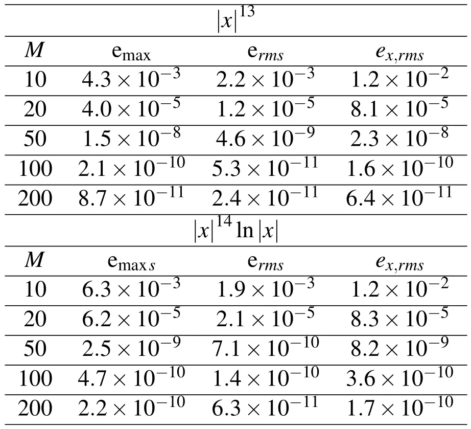
Table 3:Example 2.The maximum absolute errors emaxand RMS errors ermsin the solution of the BVP with the mixed boundary conditions(28),(29),(30)by the direct scheme of SAMM by using the RBFs as the basis functions.
?
The computational domain is a peanut shape domain with the boundary de fined by the parametric equation:
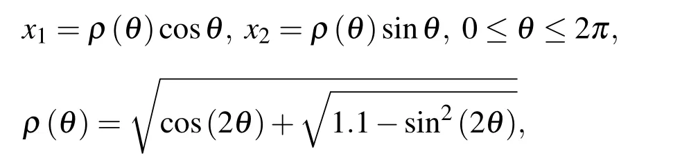
where(ρ,θ)are polar coordinates.The domain is shown in Fig.5.
The boundary conditions are of the two types:

where∂ΩDand∂ΩNare the boundaries subjected to Dirichlet and Neumann boundary conditions respectively.The portion of boundary above thex1axis has the Dirithlet boundary condition and the other portion of the boundary has the Neumann boundary condition.The functionsf(x),gD(x)andgN(x)correspond to the exact solution:


Figure 3:Example 3.The ameba-shape domain.The collocation points xnfor approximation PDE are shown inside the domain and the collocation points yifor approximation the correcting functions ωmare placed on the boundary ∂ Ω.
The data placed in Table 6 show the RMS errors in the solution of(33),(34),(35)by using the RBFsas the basis functions.The same problem was considered by Chen at all Chen,Fan and Wen(2011)using the method of particular solutions(MPS)and Kansa’s method.The better results in solution this BVP presented there are:ni=317,nb=150:erms=8.95×10⁻⁶,ex,rms=9.98×10⁻⁵-for the MPS anderms=6.64×10⁻⁷,ex,rms=1.21×10⁻³-for Kansa’s method.The right part of the table contains the data corresponding to the small parameterγ=0.001 as a multiplier before the Laplace operator.Such problems are more difficult for numerical simulation.
Table 4:Example 3.The maximum absolute errors emaxand RMS errors erms,ex,rmsin the solution of the BVP(31),(32)by using the RBFs

Table 4:Example 3.The maximum absolute errors emaxand RMS errors erms,ex,rmsin the solution of the BVP(31),(32)by using the RBFs
?
3.2 Three dimensional case
The functions

form a complete orthogonal system in the cube
Choosingαlarge enough to satisfy Ω⊂Ωα,we look for the correcting functions in the form:

The number of terms in the sum(36)and the number of unknownspm,kis:KI=the number of the different trigonometric products
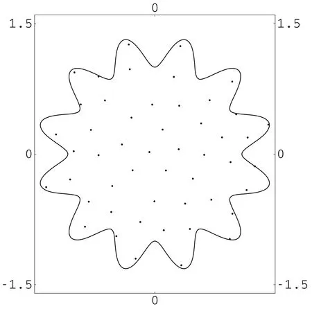
Figure 4:Example 3.The gear wheel shape domain.The collocation points xnfor approximation PDE are shown inside the domain.
withk1+k2+k3≤I.We useI=14 and soKI=364 in the calculations presented in this section.Using the collocation procedure we get the linear system:and obtain the system


Table 5:Example 3.The maximum absolute errors emaxand RMS errors erms,ex,rms in the solution of the BVP(31),(32)in the gear wheel shape domain by using the RBFs
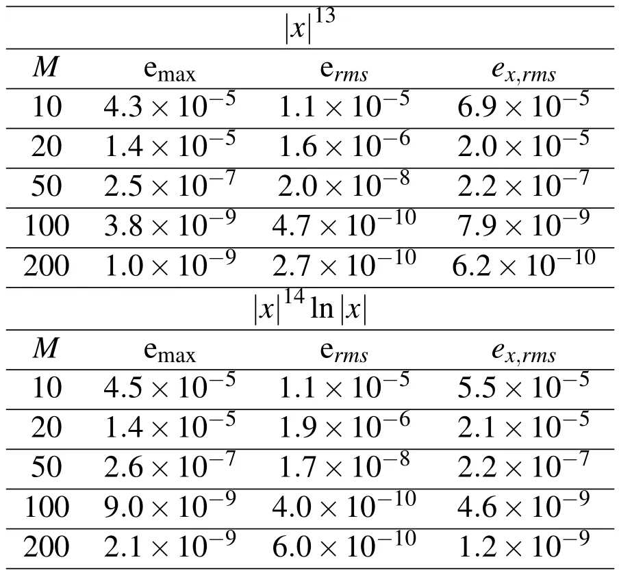
Table 5:Example 3.The maximum absolute errors emaxand RMS errors erms,ex,rms in the solution of the BVP(31),(32)in the gear wheel shape domain by using the RBFs
?
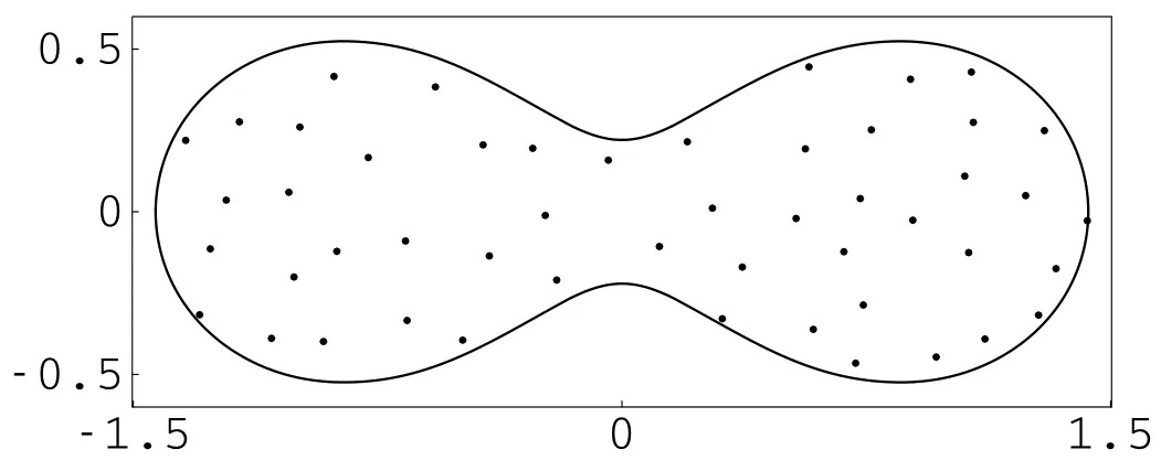
Figure 5:Example 4.The peanut shape domain.The collocation points xnfor approximation PDE are shown inside the domain.
Table 6:Example 4.RMS errors ermsin the solution of the BVP(33),(34),(35)by using the RBFs
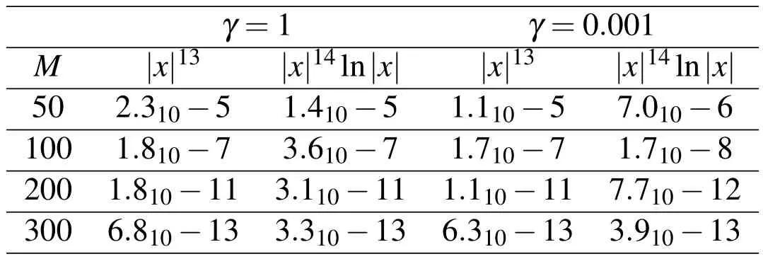
Table 6:Example 4.RMS errors ermsin the solution of the BVP(33),(34),(35)by using the RBFs
?
The solution domain is a sphere with the radiusR=1.The functionsfandgcorrespond to the exact solution:

Some results of the calculations are shown in Table 7.The parameterα=11.0 is used in all the data presented in the table.
Consider the same PDE(40)with the mixed boundary conditions on the sphere:

Here∂ΩNis the surface of the top hemispherez>0 and∂ΩDcorresponds toz<0.The functionsf(x),gD(x)andgN(x)correspond to the exact solution(42).
To calculate the RMS errorsemax,erms,ex,rmswe use the formula(25)withNt=1000 except the caseM=500,whereNt=2000 the test points are used.
Table 7:Example 5.3D problem.RMS errors ermsin the solution of(40),(41)by using the RBFs

Table 7:Example 5.3D problem.RMS errors ermsin the solution of(40),(41)by using the RBFs
?
Table 8:Example 5.3D problem.The maximum absolute errors emaxand the RMS errors erms,ex,rmsin the solution of the BVP(40),(43),(44)in the sphere domain by using the RBFs
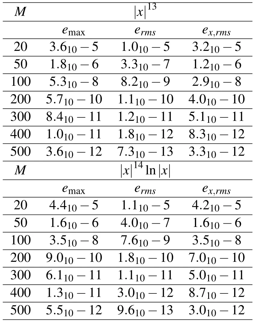
Table 8:Example 5.3D problem.The maximum absolute errors emaxand the RMS errors erms,ex,rmsin the solution of the BVP(40),(43),(44)in the sphere domain by using the RBFs
?
4 Conclusion
This paper presents a new version of the semi-analytic meshless method for solving PDEs with variable coefficients in irregular domains.The key idea of the pre-vious indirect version Reutskiy(2012,2013)is saved here:to divide satisfaction of boundary conditions and satisfaction of the governing PDE inside the domain.The new version extends the sphere of applicability of the developed technique.
While the indirect scheme permits using only such RBFswhich have the analytic solution,the novel direct scheme allows to use any smooth enough functions as the basis functions.As it is demonstrated in Example 3 and Example 5,the novel direct scheme is applicable to the PDEs with the variable coefficients in the main operator part.Besides,using the new direct scheme we can get rid of the singularities inherent to MFS and of the fictitious boundary for their placement.
The method introduced in this paper can be easily extended on to nonlinear PDEs,3D problems and time dependent problems.This will be the subject of further studies.
Abbasbandy,S.;Shivanian,E.(2011):Predictor homotopy analysis method and its application to some nonlinear problems.Commun.Nonlinear Sci.Numer.Simul.,vol.16,pp.2456–2468.
Atluri,S.N.;Liu,C.-S.;Kuo,C.L.(2009):A modified Newton method for solving non-linear algebraic equations.Journal of Marine Science and Technology,vol.17,pp.238–247.
Atluri,S.N.;Shen,S.(2002):The meshless local Petrov-Galerkin(MLPG)method:a simple&less-costly alternative to the finite element;boundary element methods.CMES:Computer Modeling in Engineering&Sciences,vol.3,pp.11–51.
Atluri,S.N.;Zhu,T.L.(1998a):A new meshless local Petrov-Galerkin(MLPG)approach in computational mechanics.Computational Mechanics,vol.22,pp.117–127.
Atluri,S.N.;Zhu,T.L.(1998b):A new meshless local Petrov-Galerkin(MLPG)approach to nonlinear problems in computer modeling and simulation.Computational Modeling and Simulation in Engineering,vol.3,pp.187–196.
Chen,C.S.;Fan,C.M.;Monroe,J.(2008):The method of fundamental solutions for solving elliptic partial differential equations with variable coefficients,in:C.S.Chen,A.Karageorghis,Y.S.Smyrlis(Eds.),The Method of Fundamental Solutions–A Meshless Method.Dynamic Publishers,Inc.,Atlanta.
Chen,C.S.;Fan,C.M.;Wen,P.H.(2010):The method of particular solutions for solving certain partial differential equations.Num.Meths Part.Diff.Eqs.,vol.33,pp.DOI:10.1002/num.20631.
Chen,C.S.;Fan,C.M.;Wen,P.H.(2011):The method of approximate particular solutions for solving elliptic problems with variable coefficients.Int.J.Comp.Meth,vol.8,pp.545–559.
Chen,C.S.;Hon,Y.C.;Schaback,R.A.(2005):Scientific Computing with Radial Basis Functions.Department of Mathematics,University of Southern Mississippi,Hattiesburg,MS 39406,USA,preprint.
Chen,W.;Fu,Z.J.;Chen,C.S.(2014):Recent Advances in Radial Basis Function Collocation Methods.SpringerVerlag.
Cheng,A.H.-D.(2000):Particular solutions of Laplacian,Helmholtz-type,and polyharmonic operators involving higher order radial basis functions.Engineering Analysis with Boundary Elements,vol.24,pp.531–538.
Cheng,A.H.-D.(2012):Multiquadric and its shape parameter-A numerical investigation of error estimate,condition number,and round-off error by arbitrary precision computation.Engineering Analysis with Boundary Elements,vol.36,pp.220–239.
Cheng,A.H.-D.;Ahtes,H.;Ortner,N.(1994):Fundamental solutions of product of Helmholtz and polyharmonic operators.Engineering Analysis with Boundary Elements,vol.14,pp.187–191.
Cheng,A.H.-D.;Cabral,J.J.S.P.(2005):Direct solution of ill-posed boundary value problems by radial basis function collocation method.Int.J.Num.Meth.Engng.,vol.64,pp.45–64.
Cho,H.A.;Golberg,M.A.;Muleshkov,A.S.;Li,X.(2004):Trefftz methods for time-dependent partial differential equations.CMES:Computer Modeling in Engineering&Sciences,vol.1,pp.1–37.
Fu,Z.J.;Chen,W.;Yang,W.(2009):Winkler plate bending problems by a truly boundary-only boundary particle method.Computational Mechanics,vol.44(6),pp.757–763.
Fu,Z.J.;Chen,W.;Yang,W.(2013):Boundary particle method for Laplace transformed time fractional diffusion equations.Journal of Computational Physics,vol.235,pp.52–66.
Golberg,M.A.;Chen,C.S.(1997):Discrete Projection Methods for Integral Equations.Computational Mechanics Publications,Southampton.
Golberg,M.A.;Chen,C.S.;Bowman,H.(1999):Some recent results and proposals for the use of radial basis functions in the BEM.Engineering Analysis with Boundary Elements,vol.23,pp.285–296.
Golberg,M.A.;Muleshkov,A.S.;Chen,C.S.;Cheng,A.H.-D.(2003):Polynomial particular solutions for certain partial differential operators.Num.Meth.Part.Diff.Eqs.,vol.19,pp.112–133.
Huang C.S.;Lee C.F.;Cheng,A.H.-D.(2007):Error estimate,optimal shape factor,and high precision computation of multiquadric collocation method.Engineering Analysis with Boundary Elements,vol.31(7),pp.614–623.
Jin,B.(2004):A meshless method for the Laplace;biharmonic equations subjected to noisy boundary data.CMES:Computer Modeling in Engineering&Sciences,vol.6,pp.253–261.
Kansa,E.(1990a):Multiquadrics–a scattered data approximation scheme with application to computational fluid dynamics,part I.Surface approximations and partial derivative estimates.Comput.Math.Appl.,vol.19,pp.127–45.
Kansa,E.(1990b):Multiquadrics–a scattered data approximation scheme with application to computational fluid dynamics,part II.Solutions to parabolic,hyperbolic and elliptic partial differential equations.Comput.Math.Appl.,vol.19,pp.147–161.
Kansa,E.;Hon,Y.(2000):Circumventing the ill-conditioning problem with multiquadric radial basis functions:applications to elliptic partial differential equations.Comput.Math.Appl.,vol.39,pp.123–137.
Larsson,E.;Fornberg,B.(2003):A numerical study of some radial basis function based solution methods for elliptic PDEs.Comput.Math.Appl.,vol.46,pp.891–902.
Li,J.;Cheng,A.H.-D.;Chen,C.S.(2003):A comparison of efficiency and error convergence of multiquadric collocation method and finite element method.Engineering Analysis with Boundary Elements,vol.27,pp.251–257.
Li,M.;Chen,W.;Tsai,C.C.(2012):A regularization method for the approximate particular solution of nonhomogeneous Cauchy problems of elliptic partial differential equations with variable coefficients.Engineering Analysis with Boundary Elements,vol.36,pp.274–280.
Li,Z.C.;Lu,T.T.;Huang,H.T.;Cheng,A.H.-D.(2007):Trefftz,collocation and other boundary methods–A comparison.Numerical Method for Partial Differential Equations,vol.23,pp.93–144.
Liu,C.-S.(2009):Fictitous time integration method for a quasilinear elliptic boundary value problem,de fined in an arbitrary plane domain.CMC:Computers,Materials&Continua,vol.11,pp.15–32.
Liu,C.-S.;Atluri,S.N.(2008a):A novel time integration method for solving a large system of non-linear algebraic equations.CMES:Computer Modeling in Engineering&Sciences,vol.31,pp.71–83.
Liu,C.-S.;Atluri,S.N.(2008b):A fictitious time integration method(FTIM)for solving mixed complementarity problems with applications to non-linear optimization.CMES:Computer Modeling in Engineering&Sciences,vol.34,pp.155–178.
Liu,C.-S.(2006):The Lie-Group Shooting Method for Nonlinear Two-Point Boundary Value Problems Exhibiting Multiple Solutions.CMES:Computer Modeling in Engineering&Sciences,vol.13,pp.149–163.
Liu,C.-S.(2007a):A meshless regularized integral equation method for Laplace equation in arbitrary interior or exterior plane domains.CMES:Computer Modeling in Engineering&Sciences,vol.19,pp.99–109.
Liu,C.-S.(2007b):A MRIEM for solving the Laplace equation in the doublyconnected domain.CMES:Computer Modeling in Engineering&Sciences,vol.19,pp.145–161.
Power,H.(2002):A comparison analysis between unsymmetric and symmetric radial basis function collocation methods for the numerical solution of partial differential equations.Comput.Math.Appl.,vol.43,pp.551–583.
Reutskiy,S.Yu.(2012):A novel method for solving one-,two-and three dimensional problems with nonlinear equation of the Poisson type.CMES:Computer Modeling in Engineering&Sciences,vol.87(4),pp.355–386.
Reutskiy,S.Yu.(2013):Method of particular solutions for nonlinear Poisson-type equations in irregular domains.Engineering Analysis with Boundary Elements,vol.37(2),pp.401–408.
Sladek,J.;Stanak,P.;Han,Z-D.;Sladek,V.;Atluri,S.N.(2013):Applications of the MLPG Method in Engineering&Sciences:A Review.CMES:Computer Modeling in Engineering&Sciences,vol.92(5),pp.423–475.
Tsai,C.C.(2008):Particular solutions of Chebyshev polynomials for polyharmonic and poly-Helmholtz equations.CMES:Computer Modeling in Engineering&Sciences,vol.27,pp.151–162.
Tsai,C.C.;Cheng,A.H.-D.;Chen,C.S.(2009):Particular solutions of splines and monomials for polyharmonic and products of Helmholtz operators.Engineering Analysis with Boundary Elements,vol.33,pp.514–521.
Tsai,C.C.;Liu,C.-S.;Yeih,W.C.(2010):A Fictitous time integration method of fundamental solutions with Chebyshev polynomials for solving Poissone-type nonlinear PDEs.CMES:Computer Modeling in Engineering&Sciences,vol.56,pp.131–151.
Tsai,C.C.;Lin,Y.C.;Young,D.L.;Atluri,S.N.(2007):Investigations on the accuracy and condition number for the method of fundamental solutions.CMES:Computer Modeling in Engineering&Sciences,vol.19,pp.103–114.
Wei,X.;Chen,W.;Fu,Z.-J.(2013):Solving inhomogeneous problems by singular boundary method.Journal of Marine Science and Technology,vol.21(1),pp.8–14.
Young,D.L.;Chen,K.H.;Chen,J.T.;Kao,J.H.(2007):A modified method of fundamental solutions with source on the boundary for solving Laplace equations with circular and arbitrary domains.CMES:Computer Modeling in Engineering&Sciences,vol.19,pp.197–222.
Zhu,T.;Zhang,J.;Atluri,S.N.(1998a):A meshless local boundary integral equation(LBIE)method for solving nonlinear problems.Computational Mechanics,vol.22,pp.174–186.
Zhu,T.;Zhang,J.;Atluri,S.N.(1998b):A meshless numerical method based on the local boundary integral equation(LBIE)to solve linear and non-linear boundary value problems.Engineering Analysis of Boundary Element,vol.23,pp.375–389.
