WENG Peixuan

(School of Mathematical Sciences, South China Normal University, Guangzhou 510631,China)

MethodofConstructingUpper-LowerSolutionsforWaveProfileSystemswithQuasi-Monotonicity

WENG Peixuan*

(School of Mathematical Sciences, South China Normal University, Guangzhou 510631,China)

The wave profile systems corresponding to a reaction-diffusion system and an integro-partial differential system withn(>1) equations and quasi-monotonicity are considered. By analyzing the principal eigen-value and eigen-vector, a constructing method of upper-lower solutions for the wave profile systems is given. Some examples to illustrate the applications of our method are given.

Keywords： reaction-diffusion system; integro-partial differential system; quasi-monotonicity; wave profile system; upper-lower solutions

A classic system of reaction-diffusion equations is the following system called KPP type

(1)

and a typical system of integro-partial differential equations is of the form

(2)

Let [0,K] be an vector interval inn.fsatisfies so call quasi-monotonicity on [0,K] if

(QM1) there exists a matrixβ=diag(β1,β2,…,βn) withβi≥0 such that

f(u)-f(v)+β(u-v)≥0(0≤v≤u≤K).

One can also define thatFsatisfies so call quasi-monotonicity on [0,K] if

(QM2)F(u,w) is nondecreasing inw, and there exists a matrixβ=diag(β1,β2,…,βn) withβi≥0 such that

F(u,w)-F(v,w)+β(u-v)≥0(0≤v≤u≤K).

As we know, that systems like (1)～(2) are models arising from many real problems with temporal-spatial variation, such as those in epidemiology, ecology, biology, chemistry and physics[1-7]. System (2) is referred as nonlocal systems, and correspondingly (1) a local diffusion system. The main reason for the name of “nonlocal system” is that the variance radio ∂u/∂tat the locationxand timetdepend on the whole space(see, e.g. [8-14]). For these systems, one key element to the developmental process and dynamical study seems to be the appearance of traveling wave solutions. A traveling wave solution is a special solution traveling without change of shape, which has been widely studied for reaction-diffusion equations[6,15-20], integral and integro-partial differential equations[9-10,14,21].

Consider the existence of traveling wavefrontu(x,t)=φ(s) (s=x+ct) for (1) and (2). It is already known that the quasi-monotonicity off(orF) leads to a conclusion that the existence of a pair of admissible upper-lower solutions for the wave profile system guarantees the existence of traveling wavefront, the proof of which is proceeded by using the monotonic iteration method accompanied with the upper-lower solutions[6,14,18-19]. Therefore, the existence of a pair of admissible upper-lower solutions is really very important for the study of traveling wavefront. However, the construction and verification of upper-lower solutions are very challenging, some time maybe said to be extremely difficult. By our best knowledge, most works in the literature concerned on the casen=1, and the works on the construction for the upper-lower solutions forn>1 is few. The first work which constructed upper-lower solutions on integro-differential systems is from Weng & Zhao[14], and the method in which is used for reaction-diffusion systems (even in the degenerate case) by Fang & Zhao[22]. Encouraged by the works of [14,19,22-24], we try to rule out the techniques on constructing the upper-lower solutions of (1) and (2) forn>1. In this article, accompanied with the analysis of constructing method, we also give a formula for the computation of minimal wave speed of traveling wavefronts.

The organization of this paper is as follows. In Section 1, we consider the system (1), and in Section 2, we study the system (2).

1 Reaction-diffusion System

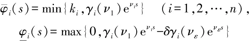
Assume that (1) has two equilibria0=(0,0,…,0)TandK=(k1,k2,…,kn)Tsuch thatf(0)=0,f(K)=0andf(u)≠0with0

(GQM1) there exists a matrixβ=diag(β1,β2,…,βn) withβi≥0 such that

f(u)-f(v)+β(u-v)≥0(-ω≤v≤u≤K),

whereω=(ω1,…,ωn)T≫0.

By substitutingu(x,t)=φ(s) (s=x+ct) into the equation (1), we obtain the wave profile system of (1):

cφ′(s)=dφ″(s)+f(φ(s)).

(3)

A traveling wavefront of (1) is a solution of (3) with monotonicity ons, satisfying

Define a wave profile set:

We now give a definition of upper-lower solutions for (3).

Definition1A continuous vector functionφ=(φ1,φ2,…,φn)Tis called an upper solution of (3) ifφis twice continuously differentiable onSand satisfies

dφ″(s)-cφ′(s)+f(φ(s))≤0

(4)

In the above definition, we do not demand that the upper-lower solutions are insideD, but we in fact construct the upper-lower solutions insideDin what follows.

1.1ConstructingMethodofUpper-lowerSolutions

In what follows, we shall mainly concern on the construction of upper-lower solutions of (3).

Note the linearized system of (1) atu=0is

(5)

whereDf(0) is the Jacobi matrix offat0. Letu(x,t)=e-νxv(t), whereν≥0 is a parameter, andv(t)=(v1(t),v2(t),…,vn(t)). Substitutingu(x,t)=e-νx×v(t) into (5), we obtain

v′(t)=ν2dv(t)+Df(0)v(t).

(6)

Consider the following matrix

γ(ν)=(γ1(ν),γ2(ν),…,γn(ν))T

express the principal eigenvector with regard toλ(ν). Thenγ(ν)>0forν≥0. In addition, in view of [25,Corollary 4.3.2], ifCνis irreducible, thenγ(ν)≫0forν≥0.

In view of the definitions of eigen-value and eigen-function, we obtain the following relation

(i=1,2,…,n,ν≥0).

(7)

Note that if λ(0)>0, then it will yieldλ(ν)>0 forν≥0.

Lemma1Assume λ(0)>0. Then the following statements are valid:

The conclusion (2) is a direct corollary from the conclusion (1) andλ(ν)>0 forν≥0.

In the following arguments, we always assume that the hypothesis (H) holds.

(1)Df(0) is irreducible;

Remark1We may in fact need ∂fi(u)/∂uj≥0 (i,j=1,2,…,n,i≠j) and -ω≤u≤Kfor some nonnegative vectorωin the practical applications.

Now we begin to state our idea of constructing upper-lower solutions of (3). For anyc>c*, in view of Lemma 1, there existν1>0 such thatΦ(ν1)=c. Here, if there exist more than oneν>0 such thatΦ(ν)=c, we always choose the smallest one, denoted asν1. Letε>0 be small andνε:=ν1+ε, such thatν1<νε<ν*and 2ν1>νε. Thus, there exists acε=Φ(νε) such thatc*

Φ(ν1)=c,Φ(νε)=cε,Φ(ν*)=c*.

(i=1,2,…,n).

(8)

ξ(s):=(ξ1(s),ξ2(s),…,ξn(s))T,

ξi(s):=γi(ν1)eν1s-δγi(νε)eνεs=

i:=ln<0 ifδ>0 is large.

We then have

ξi(i)=0,ξi(s)>0 (si).

That is, we can haveMi>0 being very small withε>0 small enough.

(9)

fi(γ1(ν1)eν1s,γ2(ν1)eν1s,…,γn(ν1)eν1s)=

fi(γ1(ν1)eν1s,γ2(ν1)eν1s,…,γn(ν1)eν1s)=

γ2(ν1)eν1s,…,γn(ν1)eν1s).

γ2(ν1)eν1s,…,γn(ν1)eν1s)≤0(s

(10)

We begin to verify the lower solution. Note the following facts:

(11)

Fors≥i, we haveφi(s)=0,φj(s)≥0 (j=1,2,…,n,j≠i) and then

(12)

Fors

δθνεγi(νε)eνεs+fi(ξ(s))=

fi(ξ(s))+δθνεγi(νε)eνεs,

whereθ=c-cε. Here we used the factφj(s)≥ξj(s) (j≠i) in (11) and Remark 1. If we use another fact in (11) thatφj(s)≥0 (j=1,2,…,n,j≠i), then we obtain

fi(0,…, 0,ξi(s),0,…,0)+δθνεγi(νε)eνεs.

Therefore, in order thatφ(s) is a lower solution of (3), we need either

fi(ξ(s))+δθνεγi(νε)eνεs≥0 (s

(13)

or

fi(0,…, 0,ξi(s),0,…,0)+δενεγi(νε)eνεs≥0

(s

(14)

Summarizing the above arguments, we obtain a conclusion as follows:

Remark2λ(0)>0 is an obvious assumptions in order to guarantee the instability of zero equilibrium, which leads to the wave propagation from zero to the positive equilibrium. Consider the cooperative system

(15)

where all constants are nonnegative. Thenλ(0)>0 is equivalent to max{r1,r2}>0.

Note that we need to substituteφn(s)≡0 into other formulas (i=1,2,…,n-1) in (13).

1.2Applications

In this subsection, we shall give two reaction-diffusion systems to illustrate the applications of conclusion (C). One system is irreducible, and another is reducible.

Example1Consider a system generalized in biochemical control circuit[25]:

(16)

wheredi>0,αi>0 andgis a bounded continuously differentiable function satisfying

M>g(v)>0,g′(v)>0 (v>0).

Typical choices ofgin the applications are

For simplicity and certainty, we consider the situation ofg(u)=u/(1+u), and thus if we assume thatα<1, then there are two equilibria of (16) as follows:

0:=(0,…,0),K:=(k1,…,kn), wherekn=1/α-1.

The corresponding form ofCνand (7) are as follows:

[λ(ν)-(d1ν2+α1)]γ1(ν)-g′(0)γn(ν)=0,

-γi-1(ν)+[λ(ν)-(diν2+αi)]γi(ν)=0

(i=2,3,…,n).

(17)

Forg(u)=u/(1+u), we haveg′(0)=1, and thusCνis irreducible.

We want to show thatλ:=λ(0)>0, and therefore, (1) in (H) is satisfied. In fact, note

detC0=(-1)nα+(-1)n+1g′(0)=(-1)n(α-1)

and det[λI-C0]=0 is equivalent to the algebra equation

p(λ):=λn+a1λn-1+a2λn-2+…+an-1λ+an=0,

wherean=p(0)=(-1)ndetC0=(-1)2n(α-1)<0. Sincep(+∞)=+∞, we know thatp(λ)=0 has positive real root, that isλ(0)>0.

Now we have

…,γn(ν1)eν1s)=eν1s[α1γ1(ν1)-g′(0)γn(ν1)]+

g(eν1sγn(ν1))-α1eν1sγ1(ν1)≤0(s

…,γn(ν1)eν1s)=eν1s[αiγi(ν1)-γi-1(ν1)]+

eν1sγi-1(ν1)-αieν1sγi(ν1)=0(s

That is, (10) is true.

We verify (13) in the following.

f1(ξ(s))+δθνεγ1(νε)eνεs=eν1s[α1γ1(ν1)-

g′(0)γn(ν1)]-δeνεs[α1γ1(νε)-

g′(0)γn(νε)]+g(eν1sγn(ν1)-δeνεsγn(νε))-

α1[eν1sγ1(ν1)-δeνεsγ1(νε)]+δθνεγi(νε)eνεs=

-g′(0)[eν1sγn(ν1)-δeνεsγn(νε)]+

g(eν1sγn(ν1)-δeνεsγn(νε))+δθνεγ1(νε)eνεs=

δθνεγ1(νε)eνεs=-e2ν1s{γn(ν1)-

δe(νε-ν1)sγn(νε)}2+δθνεγ1(νε)eνεs.

Since 2ν1>νε, we can chooseδ>0 large enough such that

-e2ν1s{γn(ν1)-δe(νε-ν1)sγn(νε)}2+

δθνεγ1(νε)eνεs≥0(s

As fori=2,…,n, we have

fi(ξ(s))+δθνεγi(νε)eνεs=eν1s[αiγi(ν1)-

γi-1(ν1)]-δeνεs[αiγi(νε)-γi-1(νε)]+

[eν1sγi-1(ν1)-δeνεsγi-1(νε)]-αi[eν1sγi(ν1)-

δeνεsγi(νε)]+δθνεγi(νε)eνεs=

δθνεγi(νε)eνεs≥0(s

The above example is the irreducible case (1) in (H). In what follows, we shall give another example which is of the reducible case (2) in (H).

Example2Consider a reaction diffusion model for competing pioneer and climax species[19]:

(18)

Assume

then we can derive thatc11c22>1 and there are two equilibria of (18) as follows:

Give another assumption for technical reason:

(P2)w*≤u*.

Letp=z0/c11-uandq=v. Then, (18) is transformed to the following system

(19)

andE1andE*are transformed to

with0andKbeing ordered and no other equilibrium between0andK, under (P1) and (P2). Notez0/c11-u*>0, thusKis a positive equilibrium.

The system (19) is a cooperative but reducible system in [0,K]. The corresponding form ofCνand (7) are as follows:

and

(20)

The two eigenvalues ofCνare

whereλ1(ν)=λ(ν) is the principal eigenvalue. Noteλ(0)>0, and the principal eigenvector corresponding toλ(ν) is (γ1(ν),γ2(ν))T, where

γ1(ν)=λ1(ν)-λ2(ν)=

Assume that there holds

(P3)d1/d2≤2.

Then we obtain by calculation that

Noting that

the assumption (P3) leads to

Summarizing the above discussion, we know that the system (19) satisfies (2) in (H).

We begin to verify (10). Fori=1 ands

e2ν1sγ1(ν1)G′(ζ(s))[c22γ1(ν1)-γ2(ν1)],

whereζ(s) is betweenz0/c11andz0/c11-γ2(ν1)eν1s+c22γ1(ν1)eν1s. Sincew*1, and we have

andc22γ1(0)-γ2(0)>0, which leads to

(21)

⟹G′(ζ(s))≤ 0,

and thus

e2ν1sγ1(ν1)G′(ζ(s))[c22γ1(ν1)-γ2(ν1)]≤0 (s

Fori=2 ands

[γ1(ν1)-c11γ2(ν1)],

we have

Therefore,

z0-c11γ2(ν1)eν1s+γ1(ν1)eν1s=

z0+[γ1(ν1)-c11γ2(ν1)]eν1s≥z0.

In view of the convexity ofF, we know thatF′(z0)

This leads to

(s

For this system, we takeφ2(s)≡0 (see Remark 3). Now, fori=1,s<1, we verify (14):

f1(ξ1(s),0)+δθνεγ1(νε)eνεs=

δθνεγ1(νε)eνεs+f1(γ1(ν1)eν1s-δeνεsγ1(νε),0)=

δθνεγ1(νε)eνεs,

whereζ(s) is betweenz0/c11andz0/c11+c22ξ1(s), which is bounded. Since |G′(ζ(s))| is bounded, and

we have from 2ν1>νεthat

ifδ>0 large enough.

In view of conclusion (C) and Remark 3, we complete the verification of upper-lower solutions for the wave profile system of (18).

2 Integro-partial Differential System

(22)

LetF(0,0)=0,F(K,K)=0, andF(u,u)≠0with0

(23)

Thus we know thatFsatisfies (QM2). In fact, for mostFwith (QM2), they may satisfies a more strong condition:

(GQM2)F(u,w) is nondecreasing inw, and there exists a matrixβ=diag(β1,β2,…,βn) withβi≥0 such that

F(u,w)-F(v,w)+β(u-v)≥0

(-ω≤v≤u≤K,ω>0).

By substitutingu(x,t)=φ(s) (s=x+ct) into the equation (2), we obtain the wave profile system of (2):

(24)

A traveling wavefront of (2) is a solution of (24) with monotonicity ons, satisfying

We also give a definition of upper-lower solutions for (24).

Definition2A continuous vector functionφ=(φ1,φ2,…,φn)Tis called an upper solution of (24) ifφis continuously differentiable onSand satisfies

(25)

2.1ConstructingMethodofUpper-lowerSolutions

Note the linearized system of (3) atu=0is

(26)

whereD1F(0,0) is the Jacobi matrix ofF(u,w) onuatu=0,w=0, andD2F(0,0) is the Jacobi matrix ofF(u,w) onwatu=0,w=0.Letu(x,t)=e-νxv(t),whereν≥0 is a parameter, andv(t)=(v1(t),v2(t),…,vn(t)). Substitutingu(x,t)=e-νxv(t) into (26), we obtain

(27)

Consider the following quasi-positive matrix

(cij(ν))n×n,

where

aij+bij(ν),

Then (27) is equivalent to the vector equation

(28)

which is a cooperative system.

(29)

Lemma2Assume that λ(0)>0 and one of the following conditions holds:

(ii)bii(0)>0 (i=1,2,…,n).

Then the following statements are valid:

(1)λ(ν)>0 (ν≥0);

ProofSinceCν≥C0, we have λ(ν)≥λ(0)>0 forν≥0 (see [25, Corollary 4.3.2]). Therefore, the conclusion (1) holds.

and hence

(30)

For fixed indexi, from the above discussion about (i) and (ii), we further know thatcij(ν)>0 for at least somej. It then follows from (29) that

By using (1) and (2), we obtain (3) directly.

(1)D1F(0,0) is irreducible, andbii(0)>0 (i=1,2,…,n);

Remark5Either (1) or (2) yields a conclusion thatCνis irreducible, and thusγ(ν)≫0forν≥0.

The following idea is similar to what in Section 2. For anyc>c*, letΦ(ν1)=c,Φ(νε)=cε,Φ(ν*)=c*,whereε>0 is small andνε:=ν1+ε, such thatc*νε.

F(K,K)=0.

-cν1γi(ν1)eν1s+Fi(γ1(ν1)eν1s,…,γn(ν1)eν1s,

(31)

We begin to verify the lower solution. Fors≥i, we haveφi(s)=0,φj(s)≥0 (j=1,2,…,n,j≠i) and then

F(0,0)=0.

Fors

-c[ν1eν1sγi(ν1)-δνεeνεsγi(νε)]+Fi(ξ1(s),

δθeνεsγi(νε)+Fi(ξ1(s),…,ξn(s),

Here we use the factφj(s)≥ξj(s) (j≠i) in (11). If we use another fact in (11) thatφj(s)≥0, then we obtain

δθeνεsγi(νε)+Fi(0,…,0,ξi(s),0,…,0,

Therefore, in order thatφ(s) is a lower solution of (24), we need either

δθeνεsγi(νε)+Fi(ξ1(s),…,ξn(s),

(32)

or

δθeνεsγi(νε)+Fi(0,…,0,ξi(s),0,…,0,

(33)

Summarizing the above arguments, we obtain a conclusion as follows.

2.2Applications

Example3Consider the following multi-type SIS epidemic model:

μiui(x,t)(1≤i≤n).

(34)

Here

F(u,w)=-μu+g(u)w,

g(u)=diag(1-u1,1-u2,…,1-un),

μ=diag(μ1,μ2,…,μn).

(H2)σj≥0,λij≥0, and the matrixΛ:=(σjλij)n×nis irreducible.

(H3) Eitherμi=0 for somei, orμ≫ 0 andρ(Γ)>1, whereρ(Γ)==max{|λ|: det(λI-Γ)=0}.

Example4In (2), if we take

F(u,w)=-u+f(u)+w,

P(y)=J(y)=diag(J1(y),J2(y),…,Jn(y)),

(35)

(1)Df(0,0) is irreducible;

Concretely, let us consider the biochemical control circuit in Example 1 withg(u)=u/(1+u):

f1(u1,…,un)=g(un)-α1u1,

fi(u1,…,un)=ui-1-αiui(i=2,…,n).

By calculation, we obtain

λ(ν)γi(ν)=ci(i-1)(ν)γi-1(ν)+cii(ν)γi(ν)=

(i=2,…,n).

(36)

Now we have

-eν1s[c11(ν1)γ1(ν1)+c1n(ν1)γn(ν1)]-

(1+α1)γ1(ν1)eν1s+g(γn(ν1)eν1s)+

g′(0)eν1sγn(ν1)≤0,

-eν1s[ci(i-1)(ν1)γi-1(ν1)+cii(ν1)γi(ν1)]-

(1+αi)γi(ν1)eν1s+γi-1(ν1)eν1s+

eν1sγi-1(ν1)=0 (i=2,…,n).

That is, (31) is true.

We verify (32) in the following. Ifi=1, we have

δθeνεsγ1(νε)+F1(ξ1(s),…,ξn(s),

-eν1s[c11(ν1)γ1(ν1)+c1n(ν1)γn(ν1)]+

δeνεs[c11(νε)γ1(νε)+c1n(νε)γn(νε)]+

δθeνεsγ1(νε)-(1+α1)[γ1(ν1)eν1s-

δeνεsγn(νε)]+g(eν1sγn(ν1)-δeνεsγn(νε))+

g(eν1sγn(ν1)-δeνεsγn(νε))-

g′(0)[eν1sγn(ν1)-δeνεsγn(νε)]+δθeνεsγ1(νε)=

(s<1)

by using the fact: 2ν1>νεandδ>0 large enough. As fori=2,…,n, we have

δθeνεsγi(νε)+Fi(ξ1(s),…,ξn(s),

-eν1s[ci(i-1)(ν1)γi-1(ν1)+cii(ν1)γi(ν1)]+

δeνεs[ci(i-1)(νε)γi-1(νε)+cii(νε)γi(νε)]+

δθeνεsγi(νε)-(1+αi)[γi(ν1)eν1s-

δeνεsγi(νε)]+[eν1sγi-1(ν1)-δeνεsγi-1(νε)]+

δeνεsγi-1(νε)≥0(s

Therefore, (32) holds.

Acknowledgments: I want to express my thanks to Professor Xiaoqiang Zhao in Memorial University of Newfoundland for his valuable discussions on the upper and lower solutions for higher dimensional (vector) systems.

[1] ARONSON D G,WEINBERGER H F. Nonlinear diffusion in population genetics, combustion, and nerve pulse propagation[M]∥GOLDSTEIN J A. Partial differential equations and related topics. Lecture notes in mathematics. New York:Springer-Verlag, 1975,446:5-49.

[2] ARONSON D G,WEINBERGER H F. Multidimensional nonlinear diffusion arising in population dynamics[J]. Adv Math,1978,30:33-76.

[3] WEINBERGER H F. Asymptotic behavior of a model in population genetics[M]∥CHADAM J. Nonlinear partial differential equations and applications. Lecture notes in mathematics. New York:Springer-Verlag, 1978,648:47-97.

[4] MURRAY J D. Mathematical biology:I & II[M]. New York:Springer-Verlag,2002.

[5] RASS L,RADCLIFFE J. Spatial deterministic epidemics[M]∥Mathematical surveys and monographs.Providence, RI:American Mathematical Society,2003.

[6] VOLPERT A I,VOLPERT Vitaly A,VOLPERT Vladimir A.Traveling wave solutions of parabolic systems[M]∥Translation of mathematical monographs. Providence, RI:American Mathematical Society,1994.

[7] WEINBERGER H F. Some deterministic models for the spread of genetic and other alterations[M]∥JGER W,ROST H,TAUTU P. Biological growth and spread. Lecture notes in biomathematics. New York:Springer-Verlag, 1981,38:320-333.

[8] AL-OMARI J F M,GOURLEY S A. A nonlocal reaction-diffusion model for a single species with stage structure and distributed maturation delay[J]. Eur J Appl Math,2005,16:37-51.

[9] BRITTON N F. Spatial structures and periodic travelling waves in an integro-differential reaction-diffusion population model[J]. SIAM J Appl Math, 1990,50:1663-1688.

[10] DIEKMANN O. Thresholds and traveling waves for the geographical spread of infection[J]. J Math Biol,1978,6:109-130.

[11] GOURLEY S A,WU J. Delayed nonlocal diffusive systems in biological invasion and disease spread[M]∥BRUNNER H,ZHAO X Q,ZOU X. Nonlinear dynamic and evolution equations, Fields Inst Commun.Providence,RI:American Mathematical Society,2006,48:137-200.

[12] SO Joseph W H,WU J H, ZOU X F. A reaction-diffusion model for a single species with age structure, I. Travelling wavefronts on the unbounded domains[J].Proc R Soc Lond A,2001,457:1841-1853.

[13] WENG P,HUANG H,WU J. Asymptotic speed of propagation of wave fronts in a lattice delay differential equation with global interaction[J].IMA J Appl Math,2003,68:409-439.

[14] WENG P,ZHAO X Q. Spreading speed and traveling waves for a multi-type SIS epidemic model[J].J Differ Equations,2006,229:270-296.

[15] SMITH H L,ZHAO X Q. Global asymptotic stability of traveling waves in delayed reaction-diffusion equations[J].SIAM J Math Anal,2000,31:514-534.

[16] WEINBERGER H F. On spreading speeds and traveling waves for growth and migration models in a periodic habitat[J].J Math Biol,2002,45:511-548.

[17] WEINBERGER H F,LEWIS M A,LI B T. Analysis of linear determinacy for spread in cooperative models[J].J Math Biol,2002,45:183-218.

[18] WU J,ZOU X. Traveling wave fronts of reaction-diffusion systems with delay[J].J Dyn Differ Equ,2001,13:651-687.

[19] YUAN Z H,ZOU X F. Co-invasion waves in a reaction diffusion model for competing pioneer and climax species[J]. Nonlinear Anal-RWA,2010,11:232-245.

[20] ZHAO X Q, WANG W D.Fisher waves in an epidemic model[J].Discrete Cont Dyn S:Ser B,2004,4:1117-1128.

[21] DIEKMANN O. Run for your life. A note on the asymptotic speed of an epidemic[J]. J Differ Equations,1979,33:58-73.

[22] FANG J,ZHAO X Q. Monotone wavefronts for partially degenerate reaction-diffusion systems[J]. J Dyn Diff Equat,2009,21:663-680.

[23] LI B T,WEINBERGER H F,LEWIS M A. Spreading speeds as slowest wave speeds for cooperative systems[J].Math Biosci,2005,196:82-98.

[24] LIANG X,ZHAO X Q. Asymptotic speeds of spread and traveling waves for monotone semiflows with applications[J].Comm Pure Appl Math,2007,60:1-40. Erratum: Comm Pure Appl Math,2008,61:137-138.

[25] SMITH H L. Monotone dynamical systems: An introduction to the theory of competitive and cooperative systems[M]∥Mathematical surveys and monographs. Providence, RI:American Mathematical Society,1995.

[26] BROWN J,CARR J. Deterministic epidemic waves of critical velocity[J]. Math Proc Cambridge Philos Soc,1977,81:431-433.

2013-03-11

国家自然科学基金项目(11171120);教育部博士点基金项目(20094407110001);广东省自然科学基金项目(10151063101000003)

1000-5463(2013)06-0006-13

O175.2; O175.6; O175.1

A

10.6054/j.jscnun.2013.09.002

拟单调波轮廓方程组构造上下解的方法

翁佩萱*

(华南师范大学数学科学学院, 广东广州 510631)

研究了空间维数n>1情形下对应于拟单调反应扩散系统和积分-偏微分系统的波轮廓方程组. 通过分析主特征值和主特征向量，给出了构造上下解的方法和一些应用例子.

反应扩散方程组; 积分-偏微分方程组; 拟单调; 波轮廓方程组; 上下解

*通讯作者:翁佩萱，教授，Email: wengpx@scnu.edu.cn.

【中文责编：庄晓琼 英文责编：肖菁】