Mohammad SOLTANIASL*, Kiyosi KAWANISI, Junki YANO, Kazuhiko ISHIKAWA

Department of Civil and Environmental Engineering, Graduate School of Engineering, Hiroshima University, Higashi-Hiroshima 739-8527, Japan

Variability in salt flux and water circulation in Ota River Estuary, Japan

Mohammad SOLTANIASL*, Kiyosi KAWANISI, Junki YANO, Kazuhiko ISHIKAWA

Department of Civil and Environmental Engineering, Graduate School of Engineering, Hiroshima University, Higashi-Hiroshima 739-8527, Japan

In this study the sub-tidal and intra-tidal variations of salt fluxes in the upstream section of a shallow estuary (with a water depth of less than 3 m) were investigated. The salt fluxes were estimated based on the cross-sectional average salinity and velocity measured by the fluvial acoustic tomography system (FATS). The results indicate that the magnitude of seaward fluxes is approximately two times greater than that of landward fluxes under normal conditions. The results of short-term observation in the study area indicate that there is a phase lag of the bottom and surface salinities between the regions with the largest and smallest depths. The vertical shear flux with a peak value of −0.7 m2/s during the ebb tide indicated an important contribution to the total salt flux compared with the advective flux. A phase lag occurred between the vertical shear terms in the regions with the largest and smallest depths, which resulted from the correlation between the vertical variations of the salinity and velocity and the existence of transversal velocity circulations.

salt flux; circulation; fluvial acoustic tomography system (FATS); Ota River Estuary

1 Introduction

Salt transport in an estuary is mainly to keep a balance between the seaward advective and landward dispersive fluxes. To date, a great number of field studies have been conducted to calculate the advective and dispersive salt fluxes within estuarine systems characterized by very low to high rates of freshwater discharge (5 to 5 000 m3/s) and mean water depth ranging from 3 to 20 m (Fischer 1972; Hughes and Rattray 1980; Uncles et al. 1985; Kjerfve 1986; Restrepo and Kjerfve 2002; Sylaios et al. 2006; Gong and Shen 2011). Fischer (1972) decomposed the longitudinal flux to distinguish between transverse and vertical effects, but without including the tidal variation of the cross-sectional area, which can be very significant in shallow estuaries with a large tidal range. Hughes and Rattray (1980) applied an improved formulation to the Columbia River Estuary. Kjerfve (1986) found seaward transport through ebb channels and landward transport through mid- and flood channels within the North Sea Inlet, in South Carolina, USA. Restrepo and Kjerfve (2002) investigated salt fluxes through three distributaries within the San Juan River Delta (Columbia) and found that advection andtidal pumping were the dominant processes in salt transport. Sylaios et al. (2006) also identified advection as the main mechanism for salt transport, which was consistently landward. Recently, Gong and Shen (2010) investigated the variability of salt fluxes at the Modaomen Estuary by numerical simulation. The mixing process in estuaries acts mainly in the longitudinal direction. Therefore, a large number of points in cross-sections should be monitored in order to obtain sufficient information. However, in most of the previous studies, the salt fluxes were estimated using the measurements of current and salinity at a few points of a cross-section at one or more stations in a particular estuary. Insufficient data significantly decreases the accuracy of the decomposition method for analyzing the mixing process. Recently, a new method for measuring the cross-sectional average velocity and salinity, which is called the fluvial acoustic tomography system (FATS), has been developed (Kawanisi et al. 2010; Kawanisi et al. 2012). This innovative method can measure the cross-sectional salinity and velocity at a shallow tidal channel with large changes of the water depth and salinity. In this study the salt fluxes within the Ota River Estuary were estimated using FATS measurement data from January to February, 2012, providing an initial understanding of the physical processes in the study area, which is essential to the proper management of water resources in the region. Furthermore, this study contributes to a greater understanding of the physical processes occurring within shallow estuarine systems.

2 Study area

The Ota River Estuary is located in Hiroshima City, Japan. The Ota River bifurcates into two main branches about 9 km upstream from the estuary mouth: the Old Ota River and the Ota Diversion Channel (Fig. 1). The freshwater runoff into the Ota Diversion Channel and Old Ota River is usually controlled by an array of floodgates, located near the bifurcation. The Oshiba Floodgate, located in the Old Ota River, consists of a fixed weir and a movable weir with three gates (Fig. 1). These gates are always completely open. The Gion Floodgate, which is located in the Ota Diversion Channel, consists of three movable sluice gates, of which, usually, only one sluice gate is open slightly. The inflow discharge is about 10% to 20% of the total discharge of the Ota River in normal conditions (Kawanisi et al. 2010). The flow at the Yaguchi Station, which is located 14 km upstream from the mouth, is not tidally modulated. The freshwater discharge before the bifurcation can be estimated using the rating curves at this station. The water level fluctuations were measured at the mouth of the Ota Diversion Channel (Kusatsu Station) and near the bifurcation of the Ota River (Gion Station). During flood events, when the discharge at the Yaguchi Station is over 400 m3/s, all sluice gates of the Gion Floodgate are completely open. The upstream border of the tidal compartment, which shows the influenced distance of the tides, is located about 13 km upstream from the mouth (Fig. 1). The tides are primarily semidiurnal, but mixed with a diurnal component. The tidal range at the mouth (Kusatsu Station) varies in a range from 0.3 m to 4 m during neap and spring tides.

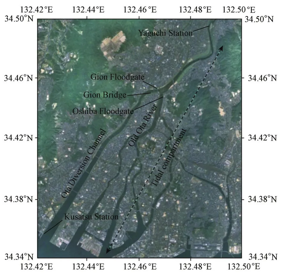
Fig. 1 Sketch of study area

3 Instruments and methods

3.1 Measurement principles of FATS

The measurement principle of FATS is the same as that of an acoustic velocity meter (AVM), which is used to calculate the cross-sectional average velocity along the transmission line using the travel time method. In other words, FATS can estimate the cross-sectional average velocity using multi-ray paths which cover the cross-section. As presented in Fig. 2, a couple of FATS’ transducers (OA and OB) with a central frequency of 30 kHz were installed diagonally on both sides of the Ota Diversion Channel near the Gion Bridge to continuously measure the cross-sectional average velocity and salinity. Based on the measurement principle of FATS, the cross-sectional average velocity (v) in the direction of stream flow is estimated with the following formula:

whereuabis the velocity along the ray path, andθis the angle between the ray path and the stream flow direction, which was 30° for these observations. The mean discharge across the cross-section at the study site was calculated as

whereA(h) is the area of the cross-section along the ray path, andhis the water depth. The cross-sectional average salinity (s) can be estimated from the sound speed measured by FATS, and the temperature and water depth (Medwin 1975):

wheretis the temperature (℃), andcis the sound speed (m/s).

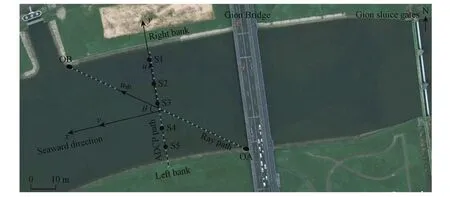
Fig. 2 Distribution of measurement cross-sections and transducers

3.2 Decomposition of salt flux

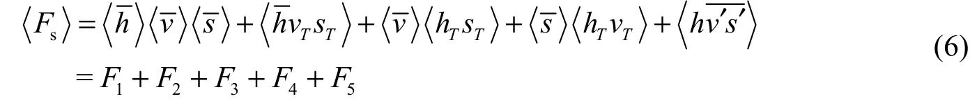
In general, the total salt flux per cross-sectional width (Fs) can be estimated as

whereTis the tidal cycle, which is assumed to be 25 hours for this study; andzis the vertical coordinate.vandswere decomposed asandwhereandare the depth-averaged longitudinal velocity and salinity, respectively, andv′ ands′ are the vertical deviation components from the depth-averaged longitudinal velocity and salinity, respectively. The depth-averaged quantities were decomposed into tidally-averaged and time-varying components as follows:

3.3 Observations

The observation site is located 245 m downstream of the Gion Floodgate (Fig. 1). Based on bathymetry data from the Japanese Ministry of Land, the mean depth, width, and bed slope of the study area are about 2.3 m, 125 m, and 0.04%, respectively. The cross-section of the channel at the study site has a trapezoidal shape with a deeper zone near the left bank. The results of mean salinity and velocity, which were estimated by FATS from January 13 to February 11, 2012 (29 days), were used for analysis of salt transport variations during the spring-neap tides. Also, in order to investigate the intra-tidal variations of the salinity and velocity, we conducted an observation during the spring tide from January 25 to 26, 2012. In this observation, the current velocity was measured using a 1.2-MHz Teledyne RDI Workhorse ADCP from a moving boat. For this study, all velocity vectors, which were estimated with FATS and ADCP, were transformed to the coordinates in anx-ycoordinate system in which the seaward direction was positive (Fig. 2). The salinity profiles were obtained using an Alec Electronics Compact conductivity-temperature-depth (CTD) profiler at five stations at an equal distance. These stations, S1, S2, S3, S4, and S5, are shown in Fig. 2. It should be noted that the practical salinity adopted in this study based on the UNESCO/ICES/SCOR/IAPSO Joint Panel on Oceanographic Tables and Standards does not have units.

4 Results and discussion

4.1 Sub-tidal variations of salinity, velocity, and salt flux

Fig. 3 shows the time series of the water level (H), discharge (Q), velocity, salinity, and fluxes. As can be seen, the upstream freshwater discharge at the Yaguchi Station was less than 80 m3/s. The salinity fluctuations were noticeably modulated by the spring-neap tidal variations. The semi-diurnal fluctuations of the salinity during the neap tides are greater than during the spring tides, which results from the different tidal mixing. The stronger tidal mixing (larger vertical eddy viscosity) during the spring tides damps down the salt intrusion over the whole observation period. Throughout the observation period, the advective fluxF1was entirely seaward. It generally followed the spring-neap tidal variations, and reached its peak values of 1.03 m2/s and 0.99 m2/s during the two neap tides, respectively. It was also modulated by the variations of the upstream freshwater discharge during the last period of the observation. The tidal sloshing fluxF2was directed landward over the observation period and reached its highest level, −0.4 m2/s, at the first neap tide. However, it was depressed by decreases in the salinity (e.g., on February 3, 2012).F3was always directed seaward following the same trend as the advective componentF1. The Stokes’ drift dispersion flux (F4) was directed landward, thuspushing saltwater into the estuary.F1andF3were substantial seaward salt fluxes, whereasF2andF4were the most significant mechanisms of landward salt transport during the observation period. The ratio of the seaward-directed fluxes (F1+F3) to the landward-directed fluxes (F2+F4) is presented in Fig. 3(f).

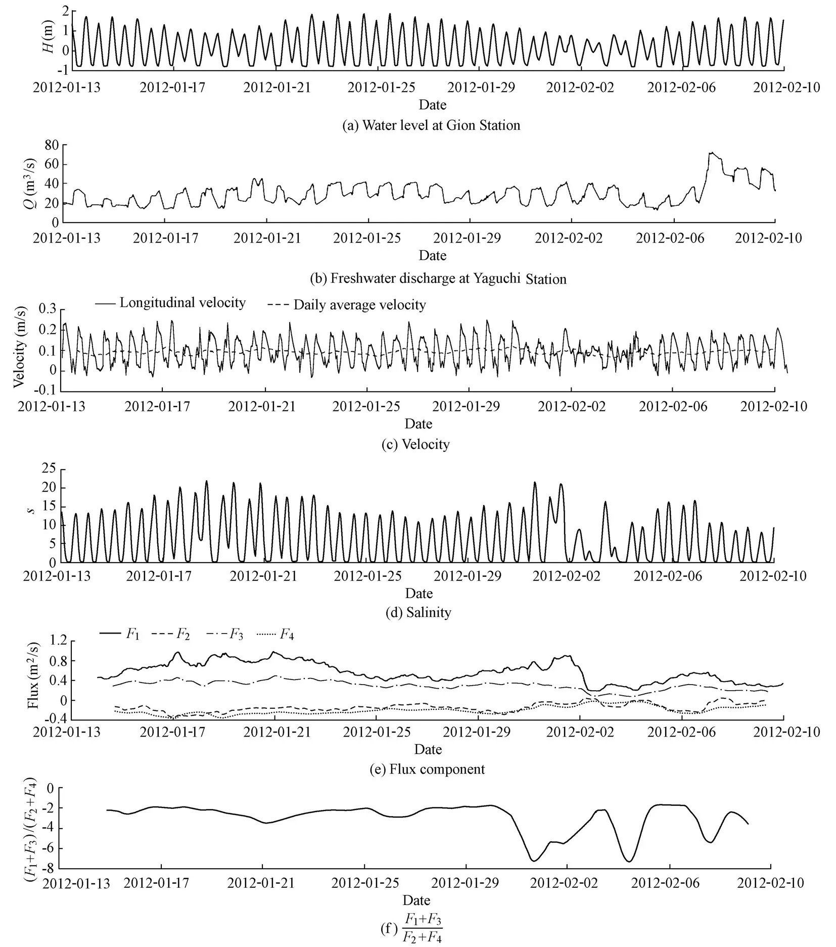
Fig. 3 Time series of water level, freshwater discharge, velocity, salinity, flux components, and

As can be seen, the magnitude of the seaward fluxes is approximately two times greater than that of the landward fluxes over the normal variations of the salinity, but this ratio increases due to decreases in the landward fluxes during the last period of the observation.These results suggest that the salt transport is predominantly controlled by the advection mechanisms during both the spring and neap tides. Moreover, both advective and dispersive fluxes are substantially more sensitive to the salinity variations than to the velocity changes.

4.2 Intra-tidal variations of salinity and velocity

Fig. 4 shows the temporal variations in the water level, salinity, mean velocity, and mean discharge, where the bottom and surface salinities shown in Fig. 4(b) are obtained from the CTD profiler, and the cross-sectional average salinity is measured with FATS. The results indicate that the differences in the mean velocity and discharge between FATS and ADCP increase during the spring tides, which may be caused by variations in the flow direction and water circulation in the study area. Stations S1 and S2 are located in front of the open sluice gate near the right bank, and station S4 is located in the region with the largest depth (Fig. 2). As can be seen in Fig. 4(b), both the bottom and surface salinities at all stations reached their highest levels after high water level conditions. The pattern of increase in the bottom salinity at all stations was similar throughout the spring tides. However, during the ebb tides the saline water in the region with the largest depth (station S4) left the cross-section around 30 minutes later than the saline water in the region with smaller depth did.

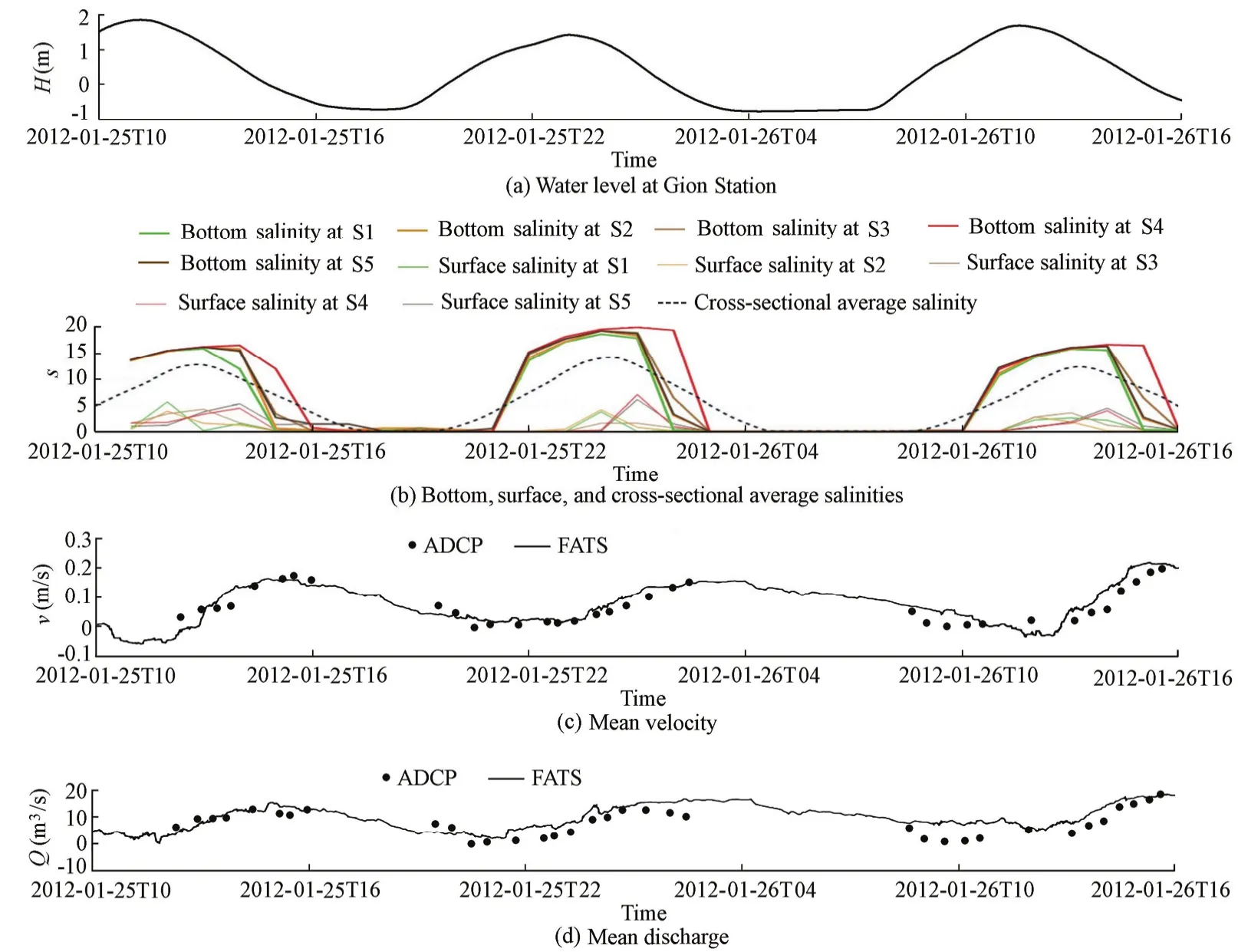
Fig. 4 Time series of water level, salinity, mean velocity, and mean discharge

The contour plots of the salinity and velocity at the cross-section along the ADCP path during the second tide are plotted in Fig. 5 and Fig. 6, respectively. At 22:00 on January 25, 2012, the current in the region withz＞ 0.25 m was directed seaward with the highest velocity of 0.11 m/s at the right bank. In contrast, in the region withz＜ 0.25 m, saline water was directed landward gradually at a velocity of around −0.15 m/s. At 23:00 on January 25, 2012, the cross-section indicates a highly stratified condition. In this situation, the velocity near the surface region is directed seaward (Fig. 6(b)). At 1:00 on January 26, 2012, the salinity was distributed throughout the cross-section. Finally, at the end of the ebb tide (at 2:00 on January 26, 2012), saltwater was limited in the region with the largest depth.

Fig. 5 Contour plots of salinity at cross-section along ADCP path during second tide

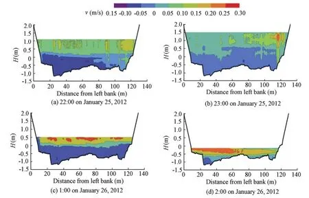
Fig. 6 Contour plots of longitudinal velocity at cross-section along ADCP path during second tide

4.3 Evaluation of stratification and shear velocity structure

Simpson et al. (1990) proposed that the degree of stratification in an estuary is determined primarily by the interaction of two competing mechanisms: the stratifying effects of tidal straining, which tend to increase stratification during the ebb tide and decrease stratification during the flood tide, and the homogenizing effects of tidal mixing which always decrease stratification. The gradient Richardson number, which represents the relative importance of gravitational circulation versus tidal mixing, is defined as

whereρis the density of water (kg/m3), andgis the acceleration of gravity (m/s2). Here, we used a dimensionless variableψ, which is called stratification parameter, to characterize the stratification variation during a tidal cycle (MacDonald and Horner-Devin 2008):

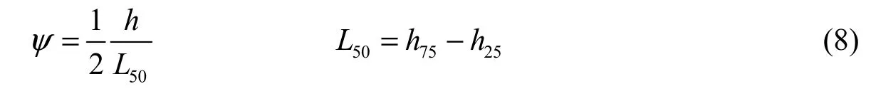
whereh75andh25are the 75th and 25th percentiles of the cross-section depth, respectively. The variation ofψthrough the second tidal cycle at five stations is presented in Fig. 7. The high value ofψat the stations at 22:00 on January 25, 2012 indicates a highly stratified situation. Throughout the ebb tideψgradually decreases and tends to a value of 1. In the region of the cross-section with the largest depth (station S4), this parameter is noticeably greater than that in the region with smaller depth throughout the whole tide. The variations ofψat the stations suggest that during the later period of the flood tide (after 22:00 on January 25, 2012) the tidal mixing contributes to the decrease of the stratification throughout the cross-section, and the stratification parameter reached its minimum at 1:00 on January 26, 2012. Eventually, during the later period of the ebb tide (after 1:00 on January 26, 2012), the stratification was enhanced by the straining process. The relative importance of the vertical velocity gradient in affecting stratification can be quantified in terms of the gradient Richardson numberRi. The variation ofRithrough the second tidal cycle is presented in Fig. 8. At hour 22:00 on January 25, 2012, in the upper layer with ds/dz＜ 0.5, which is separated by a pycnocline, and around the mid-depth of the channel withz≈ 0, the value ofRiis small.Ritends toward large values in the lower layer due to an increase in the density of water and a decrease in the velocity gradient. In the high water level situation (at 23:00 on January 25, 2012), the region with low values ofRinear the surface of the right bank is caused by the greater velocity gradients. However, at the left bank,Riis large. The temporal variations in the vertical salinity gradient over the whole cross-section are approximately equal, so the variation in the velocity distribution at the cross-section plays an important role in the variation ofRi. From 1:00 to 2:00 on January 26, 2012, the magnitudes ofRinear the boundary layer of the upper seaward and the lower landward flow (the depth is about 0.5h) vary around 0.25, while, in the near-bottomlayer,Risignificantly increases due to the higher density of water and lower values of the velocity gradient.

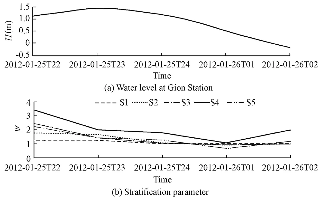
Fig. 7 Variations of water level at Gion Station and stratification parameter at five stations

Fig. 8 Transverse variations of gradient Richardson numberRiduring second tide

4.4 Variations in velocities and flux components

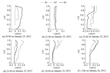
Fig. 9 Vertical profiles of longitudinal velocity measured with ADCP

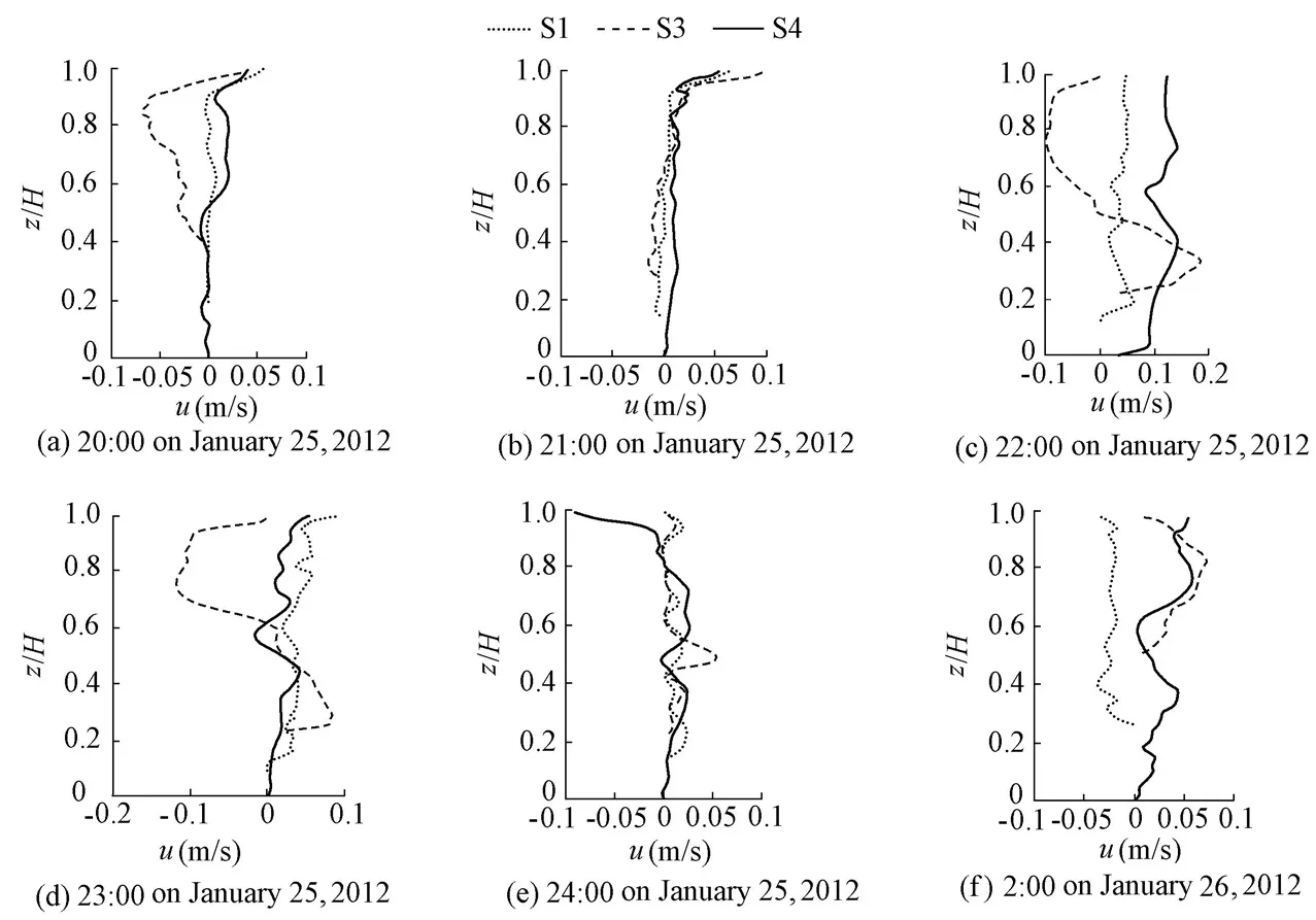
Fig. 10 Vertical profiles of transversal velocity measured with ADCP

Fig. 11 Vertical profiles of salinity measured with CTD profiler

Figs. 9, 10, and 11 show the vertical profiles of the longitudinal and transversal velocities and salinity at stations S1, S3, and S4 during the second tidal cycle. At 20:00 on January 25, 2012, the longitudinal velocityvin the region with the largest depth (station S4) shows a seaward movement throughout the water column, having a maximum value of 0.17 m/s near the surface. Meanwhile, in the region with the smallest depth (station S1) the longitudinal velocity is almost zero. This behavior is mostly associated with the freshwater flow, which enters the observation site during the ebb tide. At 21:00 on January 25, 2012, the longitudinalvelocity is completely directed landward over the whole cross-section, and the landward flow is enhanced in the region with the largest depth at 22:00 on January 25, 2012. The contribution of the transversal component of the velocity noticeably increased during the last period of the flood tide (from 22:00 to 23:00 on January 25, 2012). As can be seen in Fig. 10, this component at the center area of the cross-section (station S3) increases to its highest value near the surface and the bottom regions of the water column. This result suggests that the upward flow has a tendency to deviate towards the right bank of the channel (the front of the open sluice gate), especially in the region of the study site with the largest depth (station S4). In the high water level situation (at 23:00 on January 25, 2012) the seaward flow is reinforced in the region with the smallest depth. After that, the seaward flow in the upper layer of the water column gradually moves into the region with the largest depth. However, in the lower layer of the water column the velocity is significantly diminished. These characteristics suggest that the transversal variations in the velocity are significant at the study site, due to both the effect of the local bathymetry conditions and the interaction between the upstream gravitational and downstream tidal forces.

Fig. 12 shows the variations of the advective and vertical shear fluxes, which were estimated using the ADCP and Compact CTD data. The results indicate that the vertical shear fluxes at both station S1 and station S4 directed landward during the observation period, and the contribution of the vertical shear flux to the total salt flux, compared with the advective flux, was noticeable. In addition, there was a significant difference in the variations of the vertical shear fluxes between the regions with the largest and smallest depths. As can be seen in Fig. 12, the vertical shear flux increased to its highest level of −0.7 m2/s at station S1 at 24:00 on January 25, 2012, when the velocity in the upper layer of this region was significantly seaward. Similarly, the maximum vertical shear flux at station S4 occurred during the last period of the ebb tide, when the seaward velocity was enhanced in the region with the largest depth. Moreover, in this situation, increases in the vertical salinity gradient reinforced the vertical shear flux. These results suggest that the asymmetry in the variations of the vertical shear flux is mainly due to the high correlation between the vertical variations of the salinity and velocity and the existence of the transversal velocity circulation at the study site.

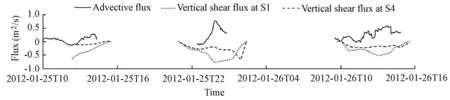
Fig. 12 Variations of advective flux and vertical shear fluxes at stations S1 and S4

5 Conclusions

In this study, the variations in salinity transport mechanisms during spring-neap tides and the intra-tidal variations in the salinity and velocity in the upstream part of the Ota RiverEstuary were investigated. The results of the salt decomposition at the study site indicated that the advective flux was entirely seaward throughout the observation period. All salt fluxes generally followed the spring-neap tidal variations during normal conditions of upstream freshwater variations. The variations in the stratification parameterψat the stations suggest that during the later period of the spring tide, the tidal mixing contributes to decreasing the stratification over the whole cross-section. The variations of the vertical shear flux indicate that this flux is directed landward during the observation period and have a significant contribution to the total salt flux compared with the advection flux. Moreover, the highest values of the vertical shear fluxes in the regions with the largest and smallest depths occur in the first and last periods of the ebb tide, respectively. These asymmetries in the highest magnitude of the shear flux are consequences of the correlation between the vertical variations of the salinity and velocity and the existence of the transversal velocity circulations.

Fischer, H. B. 1972. Mass transport mechanisms in partially stratified estuaries.Journal of Fluid Mechanics, 53(4), 671-687. [doi:10.1017/S0022112072000412]

Gong, W. P., and Shen, J. 2011. The response of salt intrusion to changes in river discharge and tidal mixing during the dry season in the Modaomen Estuary, China.Continental Shelf Research, 31(7-8), 769-788. [doi:10.1016/j.csr.2011.01.011]

Hughes, F. W., and Rattray, M. Jr. 1980. Salt flux and mixing in the Columbia River Estuary.Estuarine and Coastal Marine Science, 10(5), 479-493. [doi:10.1016/S0302-3524(80)80070-3]

Kawanisi, K., Razaz, M., Kaneko, A., and Watanabe, S. 2010. Long-term measurement of stream flow and salinity in a tidal river by the use of the fluvial acoustic tomography system.Journal of Hydrology, 380(1-2), 74-81. [doi:10.1016/j.jhydrol.2009.10.024]

Kawanisi, K., Razaz, M., Ishikawa, K., Yano, J., and Soltaniasl, M., 2012. Continuous measurements of flow rate in a shallow gravel-bed river by a new acoustic system.Water Resources Research, [doi:10.1029/2012WR012064].

Kjerfve, B. 1986. Circulation and salt flux in a well mixed estuary. Van de Kreeke, J. ed.,Physics of Shallow Estuaries and Bays, 22-29. Berlin: Springer Verlag.

MacDonald, D. J., and Horner-Devin, A. R. 2008. Temporal and spatial variability of vertical salt flux in a highly stratified estuary.Journal of Geophysical Research, 113, C09022. [doi:10.1029/2007JC004620]

Medwin, H. 1975. Speed of sound in water: A simple equation for realistic parameters.Journal of the Acoustical Society of America, 58(6), 1318-1319. [doi:10.1121/1.380790]

Restrepo, J. D. and Kjerfve, B. 2002. The San Juan Delta, Colombia: Tides, circulations, and salt dispersion.Continental Shelf Research, 22(8), 1249-1267, [doi:1016/S0278-4343(01)00105-4]

Simpson, J. H., Brown, J., Matthews, J., and Allen, G. 1990. Tidal straining, density currents, and stirring in the control of estuarine stratification.Estuaries, 13(2), 125-132.[doi:10.2307/1351581]

Sylaios, G. K., Tsihrintzis, V. A., Akratos, C., and Haralambidou, K. 2006. Quantification of water, salt and nutrient exchange processes at the mouth of a Mediterranean coastal lagoon.Environmental Monitoring and Assessment, 119(1-3), 275-301. [doi:10.1007/s10661-005-9026-3]

Uncles, R. J., Elliott, R. C. A., and Weston, S. A. 1985. Observed fluxes of water, salt and suspended sediment in a partly-mixed estuary.Estuarine, Coastal and Shelf Science, 20(2), 147-167, [doi:10.1016/ 0272-7714(85)90035-6]

(Edited by Yan LEI)

*Corresponding author (e-mail:d101090@Hiroshima-u.ac.jp)

Nov. 11, 2012; accepted May 20, 2013