YUAN Bing (袁冰)

School of Mechanical Engineering, Tianjin University, Tianjin 300072, China, E-mail: yuanbingtju@gmail.com

SUN Jian (孙健)

State Key Laboratory of Hydroscience and Engineering, Department of Hydraulic Engineering, Tsinghua University, Beijing 100084, China

YUAN De-kui (袁德奎), TAO Jian-hua (陶建华)

School of Mechanical Engineering, Tianjin University, Tianjin 300072, China

Numerical simulation of shallow-water flooding using a two-dimensional finite volume model*

YUAN Bing (袁冰)

School of Mechanical Engineering, Tianjin University, Tianjin 300072, China, E-mail: yuanbingtju@gmail.com

SUN Jian (孙健)

State Key Laboratory of Hydroscience and Engineering, Department of Hydraulic Engineering, Tsinghua University, Beijing 100084, China

YUAN De-kui (袁德奎), TAO Jian-hua (陶建华)

School of Mechanical Engineering, Tianjin University, Tianjin 300072, China

(Received June 4, 2012, Revised May 30, 2013)

A 2-D Finite Volume Model (FVM) is developed for shallow water flows over a complex topography with wetting and drying processes. The numerical fluxes are computed using the Harten, Lax, and van Leer (HLL) approximate Riemann solver. Second-order accuracy is achieved by employing the MUSCL reconstruction method with a slope limiter in space and an explicit two-stage Runge-Kutta method for time integration. A simple and efficient method is introduced to deal with the wetting and drying processes without any correction of the numerical flux term or the source term. In this new method, a switch of alternative schemes is used to compute the water depths at the cell interface to obtain the numerical flux. The model is verified against benchmark tests with analytical solutions and laboratory experimental data. The numerical results show that the model can simulate different types of flood waves from the ideal flood wave to cases over complex terrains. The satisfactory performance indicates an extensive application prospect of the present model in view of its simplicity and effectiveness.

shallow water flow, wetting and drying, finite volume method

Introduction

In the past decades, many studies were devoted to modelling shallow water flows such as estuarine and coastal flows, dam breaks and fluvial floods. A number of 2-D models were developed based on the Shallow Water Equations (SWEs) to predict the free surface flows[1-4]. Among these models, finite volume models perform quite well in view of its shock-capturing ability. However, it is still an important challenge in the numerical schemes using FVM to simulate the flooding and recession in a realistic flood inundation over irregular topography. The technique to deal with wetting and drying processes usually reflects the state of arts[5].

In finite volume models, explicit schemes are usually employed, and the SWEs are solved cell by cell. When the processes of wetting and drying are simulated, only the cells at the wet/dry interface need a special attention. Bradford and Sanders[1]addressed the wet/dry problem by considering the reconstruction near the wet/dry interface and using the velocity extrapolations instead of solving the momentum equations in these cells. In order to satisfy such properties as the C-property and the mass conservation, the numerical flux term or the source terms[4-7]were fixed in many studies, or the exact Riemann solvers[8]or the modified Riemann solvers[9]were used. The methods mentioned above are the most frequently used to deal with the wet/dry problem, among many others.

One tends to use sophisticated schemes for practical applications in the belief that the more processesa model includes, the better the model will be[10]. However, the optimal model should be the simplest that satisfies the user's need with reasonable results. Liang[5]summarized the features required for a robust flood model: ability to handle complex topography, different flow regimes including the steady or unsteady flows, subcritical or supercritical flows as well as shocks, and wetting and drying processes.

This work aims to develop a simple and efficient model for the flood simulation over complex terrain. The model neither needs to fix the flux term or the slope term, nor uses the costly exact Riemann solvers. Only a switch of alternative schemes is needed to determine the water depth at the cell interface when calculating the flux term. Thus it is simpler than most of the existing models while a similar prediction capacity can be achieved.

1. The shallow water equations

In many rivers, lakes and coastal areas, the water depth is relatively small compared to the horizontal dimension, the vertical flow can be neglected, and it is reasonable to apply the SWEs obtained by integrating the 3-D Reynolds averaged Navier-Stokes equations along the water depth. The SWEs can be written in vector form as follows

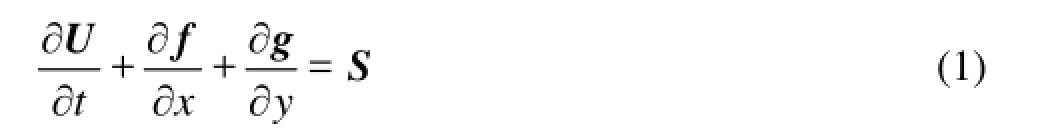
where U is the vector of conserved variables, f and g are the flux vectors in the -x and -ydirections, and S is the vector of source terms. Neglecting the Coriolis effects, the surface stress and the viscous force, the vectors U, f, g, S are given by

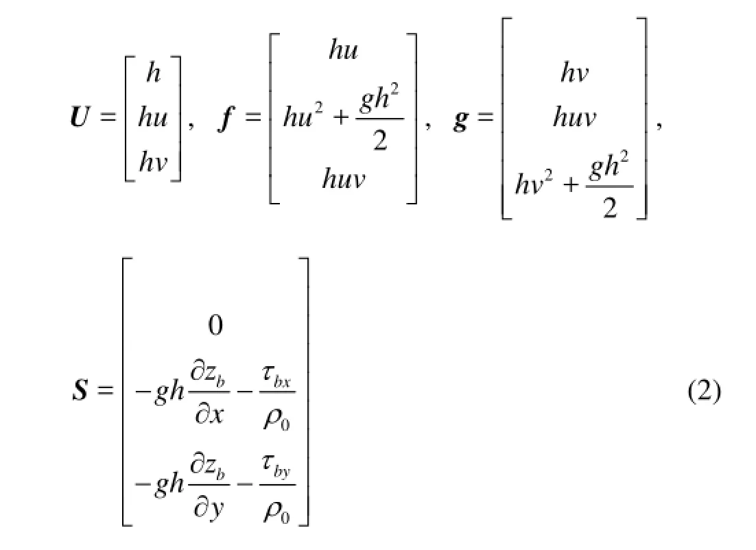
where h is the total water depth, with h=ζ-zb, ζ is the free surface elevation and zbis the bed elevation, u and v are the depth averaged velocity components in x- and y-directions, respectively, g is the acceleration of gravity,bxτ andbyτ are the bed friction stresses, ρ is the water density. The bed friction stresses are calculated by using the Chezy formula

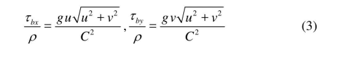
where C=h1/6/n is the Chezy roughness coefficient and n is the Manning roughness coefficient.

2. Numerical scheme

In this study, the governing equations, Eq.(1), are solved by using a cell-centered finite volume method. The numerical fluxes are calculated using the Harten, Lax, and van Leer (HLL) approximate Riemann solver. The Riemann states at each cell interface are obtained by the Monotonic Upstream Schems for Conservation Laws (MUSCL) reconstruction technique. For the time integration, a second order Runge-Kutta method is used.

2.1 Finite volume method

The study domain can be divided into a number of cells, and the conserved variables are referred to at the center of each cell. Taking a celliΩ (i is the index of cells throughout the text) as the control volume and integrating Eq.(1) over the control volume gives

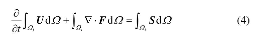
where F=(f,g) is the flux vectors. Applying the Green’s theorem to Eq.(4) gives

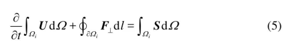
where ∂Ωiis the boundary of the cell Ωi, F⊥=F⋅n is the outward normal flux vector, n=(nx,ny) is the unit outward normal vectors on the cell edges. In the Cartesian system, it can be written as

where u⊥=unx+vnyis the normal velocity on the cell edge.

Taking an integral average of the control cells, Eq.(5) can be rewritten as

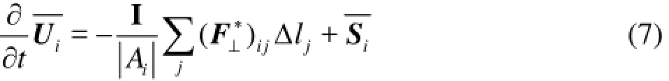
where the over-bar means the cell average value,,Ais the areaiof the cell Ωi, j is the index of the cell edges, I is a second-order unit tensor; (F⊥*)ijis the numerical flux which is computed by approximate or exact Riemann solvers, Δljis the length of the side of the cell. For simplicity, the over-bar is omitted in the following sections.

2.2 Harten, Lax, and van Leer approximate Riemann solver

In this study, the HLL Riemann solver is employed to compute the numerical flux (F⊥*)ijfor its simplicity and robustness[11]. With this solver, the numerical flux is expressed as follows (the subscripts ij are omitted for conciseness)

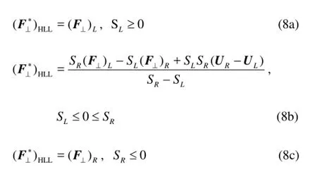
where the subscripts L and R refer to the left and right sides of the cell interfaces. The normal flux in the left and right sides, ()L⊥F and ()R⊥F, are calculated according to Eq.(6). SLandRS are the left and right wave speeds which separate the constant states of the local Riemann problem solution at the cell interface. These speeds are estimated using the Toro’s approach[12].

2.3 Monotonic Upstream Schemes for Conservation Laws (MUSCL) reconstruction

To achieve a second-order accuracy in space, the MUSCL reconstruction together with limiters is employed. The formulae with the slope limiters to compute the conserved variables at cell interfaces are as follows

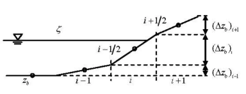
Fig.1 Scheme for domain with dry cells

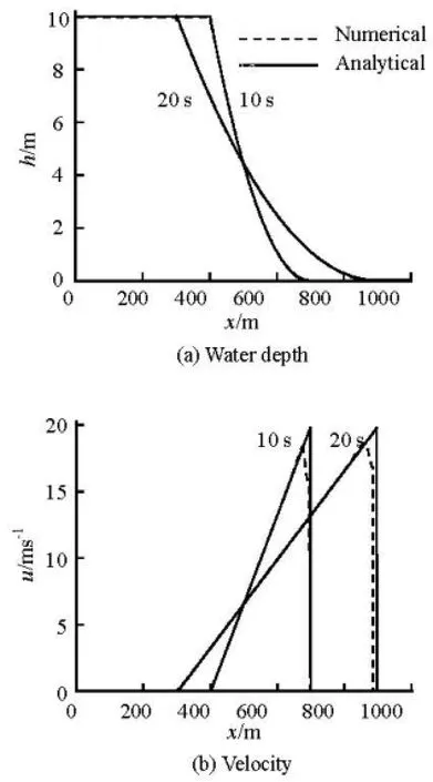
Fig.2 Comparison of analytical and numerical results for dam break over a frictionless dry bed at t=10 s and t=20 s, Δx=0.5 m

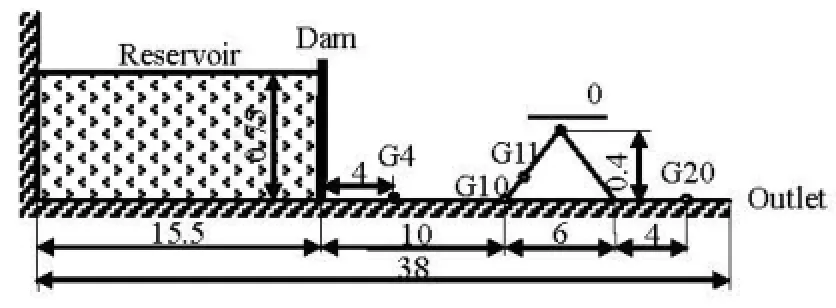
Fig.3 Side view and dimensions of the experimental dam break over a triangular obstacle (m)

Fig.4 Predicted water level of dam break over triangle obstacle at different times, =xΔ0.5 m

where ΔUi=Ui-Ui-1is the variation of a variable between adjacent cells, φ is the limiter function, rR=ΔUi+2/ΔUi+1and rL=ΔUi+1/ΔUiare the gradient ratios on the left and right sides of this cell. In this study, the structured rectangular meshes are used, so Eq.(9) is applied for both x and y directions.

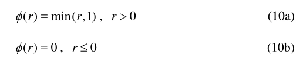
Herein the minmod limiter is used for all cases, which is of relatively low strength and is slightly dissipative. The expression of the minmod limiter is

2.4 Wet/dry boundary treatment

In the basic model, the Surface Gradient Method (SGM) proposed by Zhou et al.[11]is used in reconstruction to balance the flux gradient terms and the bed slope source terms for a wet bed. The key of the SGM is to calculate the numerical flux using the reconstructed water level instead of directly using the reconstructed depth itself, i.e.,

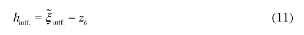
where the subscript “intf.” means the interface and the tilde “～” means the reconstructed value using Eq.(9).

It should be noted that in the SGM, the bed topography is defined at cell nodes and a piecewise linear profile is assumed within the cell, e.g., (zb)i= (zb)i-1/2+(zb)i+1/2as shown in Fig.1, and the bed slope source term should be discretized with a centered scheme to satisfy the exact C-property. The merit of the SGM is that it is as simple as the conventional method for homogeneous equations.

Actually, in the methods introduced above, it is assumed that the free surface elevation is uniform for a wet bed in a still state. Thus no matter what kind of reconstruction methods is used, after the reconstruction the value of the elevation will not change. It should be noticed that this assumption is only valid for a wet bed, for those domain with dry cells, the uniformity of the elevation could not easily be retained since the elevation for a dry bed (defined the same to thebed topography) is different from the still water level. However, the water depth for a dry bed is uniform, i.e., zero.

On the basis of the conditions mentioned above, the wet/dry interface is handled in the numerical flux calculation process in the following manner:

Firstly, the water depth at the interface of the cells is reconstructed, written asintf.(the tilde “～”means the reconstructed value and the subscript“intf.” means the interface), and

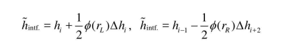
If this reconstructed water depth is less than zero, it is regarded that there is no water flow at the interface, and then the velocity and the flux are set to 0 and the reconstructed free surface elevation is set equal to the bed topography. Secondly, another water depth at the cell interface hintf.Pis calculated using an alternative approach, namely by the reconstructed elevationintf.and the relationship

If the predicted water depth is large enough, as checked by a judgment-depth h(hP＞h), the hPis used for zbintf.zbintf.calculating F⊥*, namely the original SGM is used. Otherwise, the reconstructed water depthintf.is used. The judgment-depth is determined by the following formula

where (Δzb)i(Fig.1) is the maximum difference of the topography in a cell, for a cell with a number of NS sides,, where the first number i in the subscript of zbstands for the cell number and the second number the nodes of the cell, andcrH is the critical water depth used for the judgment of wet/dry cells, and N is the total number of the cells. Since with Eq.(12), one just needs to calculate the topography difference of the nodes in the cells, without any requirement with respect to the shape of the girds, hence Eq.(12) can be applied in both one dimensional problems as well as 2-D problems, no matter the grids are structured or not. During the time integration, the water depth, the velocity and the flux are set to 0 when the water depth at the cell center is less thancrH. In the present proposed method, one just needs a switch between the predicted water depth hPand the reconstructed waterintf. depthintf.when calculating the numerical flux, and no complex modification is required for the numerical flux or the source term.

In Eq.(12), the calculation max is applied for all cells in the whole domain to obtain a uniform judgment-depth, which is convenient for comparison, however, in the real cases where the topography difference varies greatly in the study domain, the judgment-depth can be calculated just by the cells involved in the reconstruction of a certain cell, or be calculated in sub-regions divided according to the character of the topography.

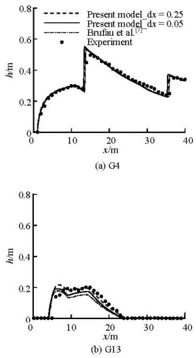
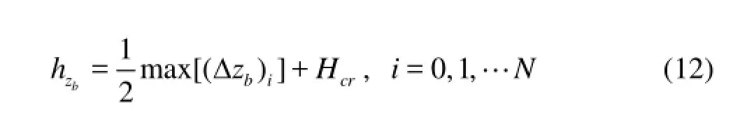
Fig.5 Dam break over triangle obstacle with different space steps: water depth at gauging points

3. Numerical tests and results

3.1 1-D dam break over dry bed

Firstly, an idealized 1-D dam break case is considered. In this test, a dam locates in the middle of a channel of 1 000 m in length and 20 m in width. The initial water depth is 10 m upstream, and 0 m downstream, respectively. Figure 2 shows the comparisons of the numerical predictions and the analytical solutions for dam break over dry bed at =t10 s and =t 20 s. It can be seen that the predicted water depth and velocity match the analytical solutions very well, which also demonstrates that the model can simulate discontinuous flows.

Fig.6 Predicted water depth and velocity of dam break over three mounds, Hcr=0.0025 m

3.2 Experimental dam break over a triangular obstacle

The model is then tested against a laboratory experimental data of a dam break over a triangular obstacle, as shown in Fig.3. This benchmark experimental test was conducted by Prof. Hiver and was cited by a number of researchers (such as in Brufau et al.[7]). The total length of the physical model is 38 m. A reservoir of 15.5 m long is located at the left side with an initial water depth of 0.75 m. A symmetrical triangular obstacle is situated 10 m downstream the dam in the dry channel. A series of gauging points of G4, G10, G11, G13 and G20 are placed along the channel. The space steps are set to 0.05 m and 0.25 m for two modeling tests, respectively, for purpose of comparison with time steps of 0.01 s and 0.05 s correspondingly.

The predicted water level variations are plotted in Fig.4, and the comparison between the predicted and measured water depth at the gauging points are shown in Fig.5. It can be seen from Fig.4(a) that at the early stage after the dam break, an expansion wave appears, and then the dry bed becomes wet in this flooding process. After the flood reaches the peak of the triangular obstacle (G13), a part of the water spills over the triangle obstacle. At the same time, the water level rises up on the slope on the upstream side of G13, and then a shock forms due to the water level difference whenthe flood wave is reflected from the slope and propagates back towards the dam (see Fig.4(b)). These features can also be seen in Fig.5 in the quantitative comparison of the predicted and measured water depth. As shown in Fig.4, the arriving times of the flood are about 1.1 s, 2.9 s, 3.2 s, 4.0 s, 6.9 s for gauging points of G4, G10, G11, G13 and G20, respectively.

As shown in Fig.5 the arriving time of the flood is well predicted at the gauging points. After the arriving times, the bed becomes wet at these points and the water depth varied due to flooding. At the point of G4, a sudden surge can be detected at time of about 13 s, which is formed at the triangular obstacle and propagates from right to left. Another surge can also be found at time of about 35 s, which is the reflected wave from the left wall. At the point of G13, the bed becomes dry at the time of about 24 s when the peak of the triangular obstacle emerges again. The comparisons show that the predictions agree generally well with the measurements, which reveals that the model can capture the major flooding feature following the dame break, including the wetting and drying processes and shock waves.

It should be pointed out that two space steps were used, i.e., =xΔ0.25 m and =xΔ0.05 m, and the predictions show good convergence. And the same predictive capability can be obtained with the coarse grid, which is very important in practical applications, especially for providing guidance on urgent responses to dam break problems.

3.3 Dam break over complex topography

To further verify the capacity of the present model in simulating floods over irregular topography, a simulation of a dam break is presented over an initially dry channel with three mounds. In this test, the dam break takes place in a closed-channel which is 75 m long and 30 m wide. The dam is located at =x 16 m. The initial water depth is 2 m between the left wall and the dam. The topography is defined as follows

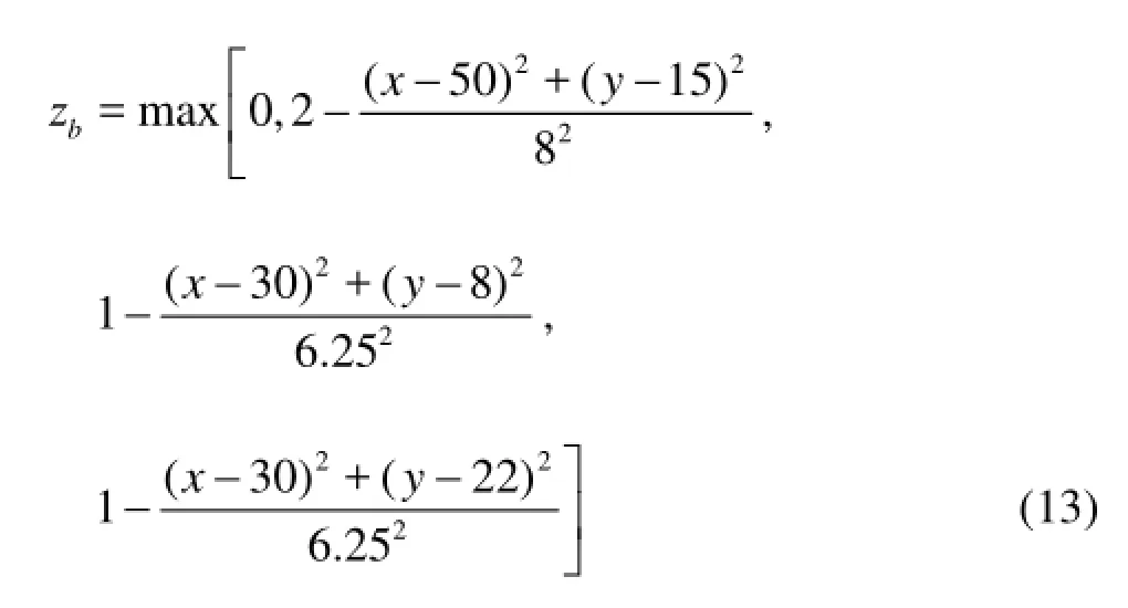
In this simulation, the space steps are 1 m both in x- and y-directions, respectively, and the time step is set as 0.1 s accordingly. The Manning roughness coefficient is set to =n0.018.

Figure 6 shows the numerical results of the free surface and the velocity at times =t2 s, 6 s, 12 s, 20 s, respectively. The dam break flood reaches the small mounds by the time =t2 s and slight surge waves can be found upstream the mounds due to the reflection by the two mounds. Until the time =t6 s, the small mounds are totally submerged by the flow and the surge waves are rising. Then the flood flows through the tall mound by the sides and reaches the downstream wall as shown at =t12 s and =t20 s, respectively. At time =t20 s, the small mounds emerge from the water while the top of the tall mound remains dry. The surge wave can be found near the left and right walls. The upstream surge is formed by the reflection of the wave against the left wall, while the formation of the downstream surge is more complex, specifically, by a wave-wall interaction as well a wave-wave interaction. The test shows that the present model can simulate the wetting and drying processes over a complex topography. Features such as wall reflection, wave-wave interaction can also be well captured.

Fig.7 Mass errors with different critical water depth for dam break over three mounds

The global mass conservation is also checked. Herein the mass error is defined by

where Mtis the total mass at time t and M0is the initial total mass. It can be seen from Fig.7 that the mass error is less than 0.11% for Hcr=0.005m and 0.06% for Hcr=0.0025m, which could meet the need for practical flow problems.

4. Discussions and conclusions

In order to simulate the wetting and drying processes such as the flooding in a dam break, a 2-D finite volume model is developed in this paper. The HLL method is used to compute the numerical flux, and the MUSCL reconstruction method and the limiting scheme are employed to achieve the second-orderaccuracy in space. A simple method is introduced to deal with the wetting and drying processes, in which a switch of alternative schemes is used to compute the water depths at the cell interface to obtain the numerical flux.

Sun and Tao[13,14]proposed a finite difference model to deal with the moving boundary problem to replace the traditional slot method[15]. In their model, the basic equations are solved by using the ADI method, in which the advection term is discretized using a central difference scheme, and the method of moving boundary is based on the linearized equations. Their model is mainly applied to the intertidal zone where the Froude Number is usually small. However, their model could not deal with the cases with a large Froude number effectively. Compared to the previous models[13-15], the present model can deal with the cases in which the Froude Number is large, such as the dam break problems, as shown by the tests in this paper. The model predictions in this paper are compared with the analytical solutions and experimental data. The results show that the model has a good shock-capturing capability and performs well in handling the wetting and drying processes. It is noticeable that the method for the wet/dry problem is simple and efficient with its good performance without any need to fix the numerical flux or the source term. Preliminary tests also show that coarse grids give satisfactory results and have the advantage of faster computation than fine grids in practice.

Acklownedgement

This work was supported by the State Key Laboratory of Hydroscience and Engineering, Tsinghua University (Grant No. 2013-ky-1).

[1] BRADFORD S. F., SANDERS B. F. Finite-volume model for shallow-water flooding of arbitrary topography[J]. Journal Hydraulic Engineering, ASCE, 2002, 128(3): 289-297.

[2] WANG Zhi-li, GENG Yan-fen and JIN Sheng. An unstructured finite-volume algorithm for nonlinear two dimensional shallow water equation[J]. Journal of Hydrodynamics, 2005, 17(3): 306-312.

[3] GUO Yan, LIU Ru-xun and DUAN Ya-li et al. A characteristic-based finite volume scheme for shallow water equations[J]. Journal of Hydrodynamics, 2009, 21(4): 531-540.

[4] HOU J., SIMONS F. and MAHGOUB M. et al. A robust well-balanced model on unstructured grids for shallow water flows with wetting and drying over complex topography[J]. Computer Methods in Applied Mechanics and Engineering, 2013, 257: 126-149.

[5] LIANG Q. Flood simulation using a well-balanced shallow flow model[J]. Journal Hydraulic Engineering, ASCE, 2010, 136(9): 669-675.

[6] CASULLI V. A high-resolution wetting and drying algorithm for free-surface hydrodynamics[J]. International Journal of Numerical Method in Fluids, 2009, 60(4): 391-408.

[7] BRUFAU P., VAZQUEZ-CENDON M. E. and GARCIA-NAVARRO P. A numerical model for the flooding and drying of irregular domains[J]. International Journal of Numerical Method in Fluids, 2002, 39(3): 247-275.

[8] PAN Cun-hong, DAI Shi-qiang and CHEN Sen-mei. Numerical simulation for 2D shallow water equations by using Godunov-type scheme with unstructured mesh[J]. Journal of Hydrodynamics, 2006, 18(4): 475-480.

[9] GEORGE D. L. Augmented Riemann solvers for the shallow water equations over variable topography with steady states and inundation[J]. Journal of Computational Physics, 2008, 227(6): 3089-3113.

[10] BATES P. D., De ROO A. P. J. A simple raster-based model for flood inundation simulation[J]. Journal of Hydrology, 2000, 236(1-2): 54-77.

[11] ZHOU J. G., CAUSON D. M. and MINGHAM C. G. et al. The surface gradient method for the treatment of source terms on the shallow water equations[J]. Journal of Computational Physics, 2001. 168(1): 1-25.

[12] TORO E. F. Shock-capturing methods for free-surface shallow flows[M]. Chrchester, UK: John Wiley and Sones, 2001.

[13] SUN Jian, TAO Jian-hua. The study on simulation of moving boundary in numerical tidal flow model[J]. Chinese Journal of Hydrodynamics, 2007, 22(1): 44-52(in Chinese).

[14] SUN Jian, TAO Jian-hua. A new wetting and drying method for moving boundary in shallow water flow models[J]. China Ocean Engineering, 2010: 24(1): 79-92.

[15] YUAN De-kui, SUN Jian and LI Xiao-bao. Simulation of wetting and drying process in depth integrated shallow water flow model by slot method[J]. China Ocean Engineering, 2008, 22(3): 1-10.

10.1016/S1001-6058(11)60391-1

* Project supported by the National Natural Science Foundation of China (Grant No. 11002099), the Tianjin Municipal Natural Science Foundation (Grant No. 11JCZDJC24200).

Biography: YUAN Bing (1987-), Male, Ph. D. Candidate

SUN Jian, E-mail: jsun@mail.tsinghua.edu.cn