SUN Ruili,LI Lei,and LI Peiliang

Physical Oceanography Laboratory,Ocean University of China,Qingdao 266100,P.R.China

1 Introduction

Long-term sea level change is an important indicator of climate change.Under the background of global climate change,global sea level is also changing correspondingly.The rising rate of sea level was approximately 1.7±0.5 mm year-1in the 20th century (Solomonet al.,2007).However,the research results based on the nearly twentyyear satellite data reveal that the rising rate of the global sea level is approximately 3.1±0.7 mm year-1(Solomonet al.,2007) and with a trend of accelerated rising.

Sea water density change caused by salinity and temperature is called the steric effect.Sea-level change caused by temperature change is called the thermosteric sea-level change,while sea-level change caused by salinity change is called the halosteric sea-level change.The sum of the thermosteric and halosteric sea level is called steric sea level.As an important part of sea level,steric sealevel changes obviously under the background of global climate warming.As pointed out in the IPCC third assessment report,an important contributor to the sea-level rise was thermal expansion,the rise rate being about 0.3–0.7 mm year-1when averaged over the 20th century.For the period 1955 –2003,the thermal expansion of the 0–700 m layer of the world ocean contributed approximately 0.3 mm year-1to the global sea-level rise (Antonovet al.,2005).The global thermosteric sea level derived from ISHII temperature data rose during 1993–2003 at a rate of 1.2 mm year-1(Zuoet al.,2010).The spatial distribution of steric sea level was also dramatically inhomogeneous with intense regional characteristics.The thermal effect accounted for 86% and 73% of the seasonal variability in the Northern and Southern Hemispheres,respectively(Zuoet al.,2009).Steric sea level,which is one of the important indicators that can characterize the distribution and content of ocean thermohaline,is related closely with global climate and possesses obvious seasonal change(Chenet al.,2001),thereby it is very meaningful to study the seasonal change of steric sea level.

It is generally believed that seasonal sea-level change reflects the seasonal fluctuations of temperature over the oceans.Many investigations (Repertet al.,1985; White and Tai,1995; Chamberset al.,1997) show that sea-level changes are highly correlated with heat storage change.The contribution of halosteric sea level to steric sea level is very small on the global scale (Antonovet al.,2002;Yanet al.,2008).In this paper,we neglect salinity effects in the steric calculation because of two considerations: 1)the lack of reliable salinity data on worldwide ocean scales; 2) the difficulties in separating the salinity variations due to ocean currents and salt convection from the salinity variations in the top of the mixing layer due to fresh water in-flux and out-flux associated with precipitation,evaporation and river discharge.The latter is caused by oceanic mass variation,which is actually part of the non-steric,or mass-related information (Chenet al.,1999).

The steric sea-level change depends on the temperature variations in the oceans at all depths (mainly in the mixing layer),which are only available fromin situobservations,such as those by XBT and MBT.Due to the inadequate spatial and temporal coverage of historicalin situmeasurements,a global real-time three-dimensional temperature field of the oceans is not available.However,if we focus on large-scale seasonal variations,the climatological temperature field based on historicalin situmeasurements will be valuable (Chenet al.,1999).We can improve the accuracy of surface temperature field by replacing the climatological temperature field with that from satellite sea surface temperature (Chenet al.,1999).

2 Data and Models

2.1 Altimeter-Grace SSL

The Altimeter-Grace SSL data (the download website:http://grace.jpl.nasa.gov/data/),which is provided by the Gravity Recovery and Climate Experiment,is composed of satellite radar altimeters data such as those from TOPEX/POSEIDON and JASON-1,and GRACE gravity data.Sea level (here meaning the absolute sea level)change consists of steric sea level change and mass-related sea-level change.Satellite radar altimeters measure the combination of both,while GRACE only measures the changes in gravity caused by local change in water mass,and water mass variations can be converted into mass-related sea-level changes.Thus altimetry and GRACE data can be combined for calculating steric sealevel change.GRACE gravity is calculated using two different smoothing radius (500 km and 750 km) for the period from February 2003 to April 2005.In this paper,we adopt the smoothing radius of 500 km.The GRACE data is continuous except for a 4-month gap between June and November 2004,and we use average annual data to make up the four-month gap.The coverage of GRACE data is 65.5˚N–65.5˚S and 0.5˚E–359.5˚E,with spatial resolution of 1˚×1˚,and time resolution of one month.

2.2 ISHII Data

The ISHII data (the download website: http://dss.ucar.edu/datasets/ds285.3/) is derived from WOA05/WOD05 data,tropical pacific thermohaline data provided by IRD,sea surface temperature data of COBE ,and ARGO data.There are sixteen layers from the top layer to the 1500 m depth (0,10,20,30,50,75,100,125,150,200,250,300,400,500,600,700,800,900,1000,1100,1200,1300,1400,and 1500 m).The time span is from January 1945 to December 2010,the spatial span being 89.5˚N–89.5˚S and 0.5˚E–359.5˚E with resolution 1˚×1˚.

2.3 OISST Data

The Optimum Interpolation SST (OISST) data are produced by combining satellite radiometer measurement,in situobservation,and the sea-ice model at the National Center for Environment Prediction (NCEP) (Reynolds and Smith,1994).The monthly OISST fields are derived by a linear interpolation of weekly optimum interpolation fields to daily fields,then the daily values are averaged over a month.Thein situdata are obtained from radio messages carried on the Global Telecommunication System,and the satellite measurements are from the operational data produced by the National Environmental Satellite,Data and Information Service (NESDIS) (Chenet al.,1999).The spatial resolution of OISST fields is 1˚×1˚ for the coverage of 89.5˚N–89.5˚S and 0.5˚E–359.5˚E.The time span is from December 1981 to December 2006.

2.4 Modified 3-D Ocean Temperature Field

Fig.1 The differences between OISST and ISHII SST in March and September.

We obtain the modified 3-D ocean temperature field by replacing the sea temperature field of the top three layers with OISST.The differences between OISST and the temperature in the top layer of ISHII in March and in September are shown in Fig.1.We can find that in most regions,the differences are less than ±1℃.However,the differences can reach ±2–4℃ in the high-latitude regions,some low-latitude regions of the Pacific,and some coastal regions.The large temperature discrepancies in the highlatitude regions in the southern hemisphere are mainly due to the sparsity of thein situdata.The ISHII climatology is estimated from all available historicalin situtemperature observations collected over a long period,while OISST seasonal average is computed from measurements of nearly three decades.The strong inter-annual and decadal SST variations will be a major error source of these discrepancies (Chenet al.,1999).In some coastal regions,the discrepancies are most likely due to the contaminated satellite data because of coastal pollution and the effects of coastal currents and some short-term phenomena.Chenet al.(1999) found by experiment that in most regions,the temperature of the top layers (0–25 m)is very close to the sea surface temperature,thereby we replace the top three layers’ temperature of ISHII with OISST in this paper.

3 The Method of Calculating the Steric Sea-Level Change

The thermal expansion coefficientCis defined as(Knauss,1996)

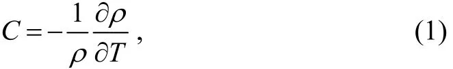
the salt compression coefficientDis defined as

in whichTis the temperature;ρis the density of seawater;CorDis a function of temperature (T),pressure (P),and salinity (S).If the thickness of the seawater layer isH,the mean temperature isT,the mean salinity isS,the mean pressure isP,∆Tis the difference between the multi-year average temperature and the monthly average temperature,and ∆Sis the difference between the multi-year average salinity and the monthly average salinity,we can obtain the thermosteric sea level by Eq.(1) under the assumption that there is no horizontal expansion

and obtain the halosteric sea level by Eq.(2)

We can obtain the total thermosteric and halosteric sealevel change at a given grid point by Eqs.(3) and (4):whereαis latitude;λis longitude;iis layer number;tis time.

4 The Comparison Between the Modified SSL and Ordinary SSL

The trend has been removed from Altimeter-Grace SSL.Therefore,we remove the trend from the modified SSL and ordinary SSL during the period from February 2003 to April 2005 in order to be consistent with Altimeter-Grace SSL.We subtract the modified SSL and ordinary SSL from the Altimeter-Grace SSL respectively and then obtain the rms errors of the difference.As shown in Fig.2,the rms errors of modified SSL and ordinary SSL are between 3cm and 5cm,and the former is obviously smaller than the latter.As shown in Fig.3,in the basin scale,the rms error of the modified SSL is obviously smaller than that of the ordinary SSL.Both are small in the Pacific Ocean while both are big in the Indian Ocean,which is likely related to the width of the basin.The width of the Pacific Ocean is the biggest and that of the Indian Ocean is the smallest.The bigger the width of the ocean is,the less contamination caused by the coastal pollution in the satellite data suffers,and the higher the accuracy of the satellite data is.

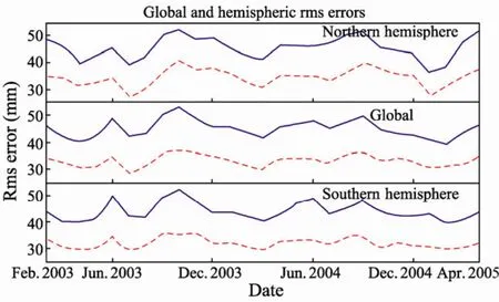
Fig.2 Rms errors for global and hemisphere scale.The blue dashed lines indicate the rms errors of the ordinary SSL; the red solid lines indicate the rms errors of the modified SSL.

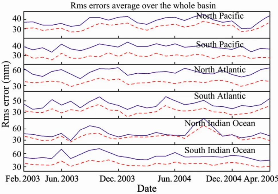
Fig.3 Rms errors in the basin scale.The blue dashed lines indicate the rms errors of the ordinary SSL; the red solid lines indicate the rms errors of the modified SSL.

We can reach the conclusion based on Figs.2 and 3:under the assumption that the Altimeter-Grace SSL is accurate,the modified SSL can reflect the true steric sea level more accurately.In the paper,we also verified the rms errors within the span of ten latitudes,and found that the rms error of the modified SSL is remarkably smaller than that of the ordinary SSL.

5 The Analysis of the Modified SSL

5.1 Secular Change

Secular change of the modified SSL was calculated with the 0–700 m ISHII temperature data and the OISST data in the past 25 years (1982–2006).

5.1.1 Global secular change

As shown in Fig.4,the global modified SSL rises obviously with a rate of 0.6mm year-1and possesses an obvious seasonal change in the period 1982–2006.The global rising rate calculated by Zuoet al.(2009),is 1.2 mm year-1during the period from 1982 to 2006.The difference may have arisen from the different time periods because the sea level rising is very fast during the period from 1993 to 2003.However,the rising trend is not monotonic: the global modified SSL rises with a rate of 0.4 mm year-1during 1982–1991 and 1.6 mm year-1during 1995–2003,while the global modified SSL descende with a rate of 0.5 mm year-1during 1992–1994 and 0.6 mm year-1during 2004–2006.The global modified SSL descende obviously since 2003,which is correlated with the sea water temperature decrease since 2003 (Solomonet al.,2007).As shown in Fig.5,the amplitude of change of the modified SSL in the northern and southern hemisphere is obviously greater than that of the modified SSL in the global ocean and the tropical region.The reason may be that the greatest change of solar radiation in both hemispheres causes the greatest amplitude of SST change(Fig.6),and then causes the amplitude of the modified SSL change in both hemispheres to be obviously greater than those in the tropical region and global ocean.The change of the modified SSL in both hemispheres is out of phase,which is associated with the solar radiation change from south to north,and the SST in the northern hemisphere is high in the summer and low in the winter,which is reversed in the southern hemisphere.In the tropical region,there is a rising rate of 0.5 mm year-1,with obvious oscillations with periods of six months,one year,and four to eight years.During 1998–1999,there is an obvious decline trend in the tropical region and the global ocean,which is likely correlated with the global sea level decline in the late stage of EI Niño (Ronget al.,2008).The rising rate is 0.3 mm year-1in the southern hemisphere,while being 1.3 mm year-1in the northern hemisphere.The latter is four times the former and the contribution of the southern hemisphere to global SSL is 52.73%.Zuoet al.(2009) proposed that the rising rate of SSL in the northern hemisphere is twice that in the southern hemisphere,and the results in this paper basically agrees with those calculated by Zuoet al.(2009).The SSL changes in the southern hemisphere and the tropical region are in phase with that of the global SSL,and their correlation coefficients are 0.61 and 0.75,respectively.The reason may be that the sea surface area of the southern hemispere accounts for a large proportion of that of the global ocean,and then the modified SSL change in the tropical region and in the global ocean is mainly modulated by that in the southern hemisphere,whose sea surface area accounts for 44.23%of the global (see Table 1).

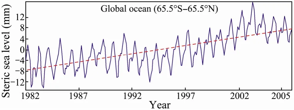
Fig.4 Modified SSL change of global ocean (65.5˚S–65.5˚N) from 1982 to 2006.The blue solid line indicates the change of the modified SSL,and the red dashed line indicate s the change trend.

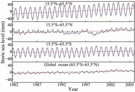
Fig.5 Global and hemispheric modified SSL change from 1982 to 2006.The blue solid lines indicate the change of the modified SSL,and the red dashed lines indicate the change trend.

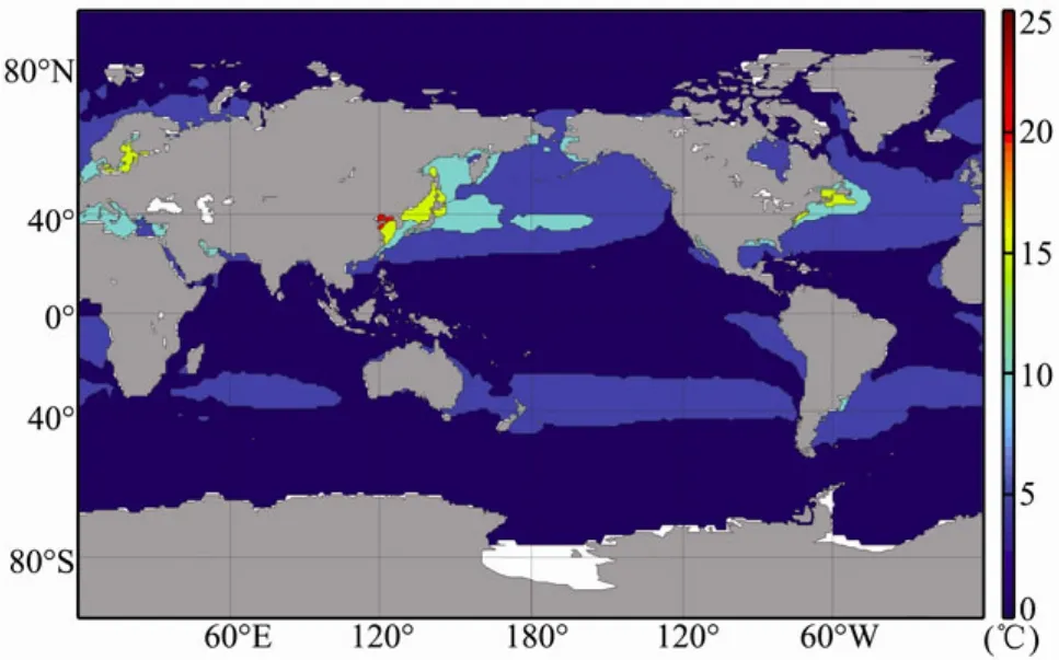
Fig.6 The distribution of the amplitude of the global SST seasonal change.

5.1.2 The secular change in the three oceans

The modified SSL changes were calculated for the South/North Pacific,South/North Atlantic,South Indian Ocean,tropical Pacific,tropical Atlantic,tropical Indian Ocean,65.5˚S–65.5˚N Pacific,65.5˚S–65.5˚N Atlantic,and 65.5˚S– 30.5˚N Indian Ocean.And the rising rates and contribution rates were also calculated.As shown in Fig.7,the change amplitudes of SSL are the greatest in the North Pacific and the North Atlantic,which may be associated with the greatest amplitude of seasonal change of the SST in the northern Pacific and northern Atlantic (see Fig.6),while the change of amplitudes of SSL are the lowest in the tropical region,the Pacific and the Atlantic.On ocean scale,the amplitude of modified SSL change in the Indian ocean is the greatest,and the reason may be that the modified SSL change in the northern hemisphere is out of phase with that in the southern hemisphere and the area of the Indian ocean is the smallest in the northern hemisphere.

During 1982–2006,the Pacific modified SSL rose with a rate of 0.7 mm year-1(Table 1) and possessed obvious six-month and one-year period oscillations,and wavelet analysis revealed that there is also 2–7 year period oscillations.The contribution of the Pacific to the global SSL is the greatest and accounts for 57.97%; The Atlantic SSL rises the fastest among the three oceans and possesses obvious 1-year period oscillations and weak 6-month period oscillations.The rising rate is 1.0mm year-1in the Atlantic ocean,accounting for 37.96% of the global modified SSL rise (Table 1) (which agrees with the results calculated by Zuoet al.(2009)),though the Atlantic accounts for only 24.3% of the total global ocean area.According to Levituset al.(2005),the heat content change takes place mainly in the upper 1000 m layer in the Atlan-tic Ocean,but only above 300 m in the Pacific and Indian Oceans.Therefore,the contribution of the Atlantic Ocean to the global SSL change should be larger.Zuoet al.(2009) proposed that the thermosteric sea level is rising very fast.The Indian ocean modified SSL rises the slowest and has obvious one-year period oscillations.The rising rate is 0.1 mm year-1,which accounts for 3.7% of the global modified SSL rise withthe smallest contribution among the three oceans.

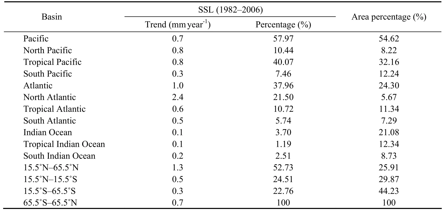
Table 1 Linear trend values of the modified SSL and the ratios in different regions

Fig.7 The modified SSL change on basin scale from 1982 to 2006.The blue solid lines indicate the change of the modified SSL,and the red dashed lines indicate the change trend.

In the northern hemisphere,the modified SSL in the Pacific and the Atlantic rises with a rate of 0.8 mm year-1and 2.4 mm year-1,respectively,and both have obvious one-year period oscillations.The North Atlantic modified SSL rises the fastest among all regionsand contributes 21.5% of the global modified SSL rise,though the North Atlantic accounts for only 5.67% of the global ocean area,which is likely due to either the heat content change in thicker sea water in the Atlantic ( Levituset al.,2005),or the sea water freshening in the North Atlantic (Solomonet al.,2007),or both.

The tropical Pacific,tropical Atlantic and tropical Indian ocean modified SSLs rise with rates of 0.8,0.6 and 0.1 mm year-1,respectively.Wavelet analysis shows that,they all possess oscillations with 6-month,1-year and interannual periods.The inter-annual oscillations in the tropical Pacific have 2–8 year period oscillations,whose correlation coefficient with SOI is 0.272,which reflects that these inter-annual oscillations are correlated with ENSO events.

The South Atlantic modified SSL rises the fastest among all regions in the southern hemisphere; however,the rising rate 0.5 mm year-1in the South Atlantic is the smallest in the whole Atlantic.And the rising rate in the South Pacific is also the smallest in the whole Pacific.However,the south Indian Ocean modified SSL rises faster than that in the tropical Indian Ocean.

5.1.3 Spatial distribution of the linear trend

The spatial distribution of the modified SSL trend during 1982–2006 is dramatically inhomogeneous with intense regional characteristics (Fig.8).The modified SSL indicates a zonal dipole in the tropical Pacific,rising in the west and descending in the east; the distribution is likely correlated with La Nina events.In the North Atlantic,the modified SSL indicates a meridional dipole,rising in the latitude band of 20˚N–40˚N and 45˚N–65.5˚N and descending obviously in the northwest region of the latitude band of 40˚N–45˚N.

In some regions (e.g.the northwest Pacific),the rising rate could reach 8.4 mm year-1,about 13 times that of the global mean.However,the descending rate in some regions in the latitude band of 40˚N–45˚N,could reach −4.0 mm year-1.The modified SSL is correlated with ocean currents such as the north and south equatorial currents in the Pacific,the extensions of the Kuroshio and Gulf Stream,and the Antarctic Circumpolar Current,i.e.,with some strong currents where the change trend of the modified SSL is obvious.

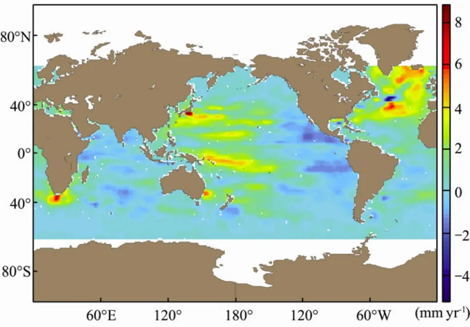
Fig.8 Distribution of the modified SSL linear trend during 1982–2006.

5.2 Spatial-Temporal of the Modified SSL

5.2.1 Global spatial-temporal change of the modified SSL

The Empirical Orthogonal Function (EOF) method was applied to the analysis of the global modified SSL.The variance contribution of the first mode is 27.08%.As shown in Fig.9,there are greater amplitudes in the latitude band of 20˚N –40˚N and the tropical region.The amplitudes of the warm pool in the west Pacific and the eastern equatorial Pacific are greater while the modified SSL in both areas is out of phase,indicating a zonal dipole.There is also a dipole in the northern Indian Ocean.As shown in Fig.10,the first mode of the modified SSL possesses an obvious seasonal change.

Fig.9 The first mode of the global modified SSL.

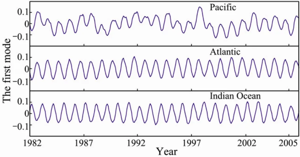
Fig.10 The time series of the first mode of the global modified SSL.

5.2.2 Spatial-temporal change of the modified SSL in the three oceans

As shown in Fig.11(a),the spatial distribution of the first mode of the Pacific modified SSL shows that the amplitudes of the modified SSLs of the tropical east Pacific and the west Pacific are greater and the modified SSLs in both areas are out of phase.In the western Pacific,the amplitudes of the modified SSL of the equatorial region and the region around 40˚N are greater and the modified SSLs in both areas are out of phase.The variance contribution of the first mode of the modified SSL in the Pacific is 24.69%.In Fig.11(c),the modified SSL in the eastern and western Indian ocean are out of phase overall and the amplitude in the equatorial region is lower.The variance contribution of the first mode of the modified SSL in the Indian Ocean is 26.93%.In the Atlantic(Fig.11(c)),the modified SSLs in the Southern and Northern Hemispheres are out of phase and the amplitudes of the modified SSLs in the regions around 40˚N and 40˚S are greater.The variance contribution of the first mode of modified SSL in the Atlantic is 40.86%.

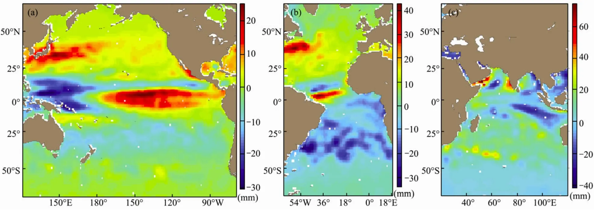
Fig.11 (a) The first mode of the modified SSL in the Pacific,(b) the first mode of the modified SSL in the Atlantic,(c)the first mode of the modified SSL in the Indian Ocean.

As shown in Fig.12,the time series of the first mode of the modified SSL in the Pacific,Atlantic and Indian Oceans all exhibit obvious one-year period oscillations.The first mode of the modified SSL in the Pacific also shows 2–6 year oscillations,whose correlation coefficient with SOI is −0.526,illustrating that the first mode of the modified SSL in the Pacific is highly correlated with ENSO events.

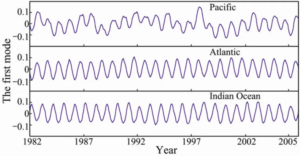
Fig.12 The time series of the first modes of modified SSL in the three oceans.

As the ENSO is a large-scale ocean-atmosphere interaction phenomenon and can influence the whole world.It can influence the SST of oceans and the modified SSL change in regions of oceans.So by finding the correlation coefficient between the time series of the first mode of modified SSL in an ocean and the corresponding indexes of El Niño,we could find to what extent is the effect of El Nino region on the main mode of the modified SSL in the ocean.From the correlation coefficients between the time series of the first mode of the modified SSL in each sea region and each EINO region index (Table 2),we can find that,from EINO1_2 to EINO4,in other words,from the tropical east Pacific to the tropical west Pacific,in the Pacific,the absolute value of the negative correlation coefficient decreases gradually and then the positive correlation coefficient increases gradually; in the Atlantic,the absolute value of the negative correlation coefficient decreases gradually and then the positive correlation coefficient increases gradually; in the Indian Ocean,the positive correlation coefficient decreases gradually and then the absolute value of the negative correlation coefficient increases gradually; in the global ocean,the absolute value of the negative correlation coefficient decreases gradually and then the positive correlation coefficient increases gradually,which shows that the correlations between each EINO region and the first mode of the modified SSL in each ocean changes gradually,either increase-ing or decreasing.

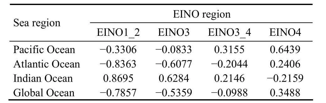
Table 2 The correlation coefficients between the time series of the first mode of the modified SSL in each sea region and each EINO region index

6 Summary

By introducing SST to the calculating of steric sea level and under the assumption that the GRACE SSL is accurate for the period 2003–2005,the accuracy of the modified SSL is obviously better than that of the ordinary SSL on different spatial scales,which shows that the modified SSL can reflect the true steric sea level more accurately.

The modified SSL in sea areas of different spatial scales exhibited an obvious rising trend in the upper 0–700 m during 1982–2006.The global mean SSL rises with a rate of 0.6 mm year-1,and the mean SSL in the Atlantic rises the fastest with a rate of 1 mm year-1among the three oceans.The SSL in the North Atlantic rises the fastest with a rate of 2.4 mm year-1.The contribution of the Pacific to the global modified SSL is the greatest,accounting for 57.97%.

The modified SSLs in sea areas of different spatial scales all possess obvious one-year period oscillations.There are 4–8 year period oscillations in the global ocean and 2–7 year period oscillations in the Pacific.Applying the Empirical Orthogonal Function method to the sea areas of different spatial scales,we find that the first modes all possess obvious 1-year period oscillations,the first mode of the modified SSL in the global ocean possesses 4–8 year period oscillations,and the first mode of the modified SSL in the Pacific possesses 2–6 year period oscillations.The correlation coefficient between the SOI index and the time series of the first mode of the modified SSL in the Pacific is −0.526,which illustrates that the first mode of the modified SSL in the Pacific is highly correlated with ENSO events.The correlation between each EINO region and the first mode of the modified SSL in each ocean changes gradually,either increasing or decreasing.

For the period 1982–2006,the spatial distribution of the linear rising trend of the global modified SSL in the upper 0–700 m is inhomogeneous with intense regional characteristics.The modified SSL linear trend indicates a zonal dipole in the tropical Pacific,rising in the west and descending in the east,which shows that the distribution is likely correlated with La Nina events.In the North Atlantic,the modified SSL indicates a meridional dipole,rising in the latitude band of 20˚N–40˚N and 45˚N–65.5˚N and descending obviously in the latitude band of 40˚N–45˚N.The modified SSL is correlated with ocean currents;for instance,there are some strong currents where the change of trend of the modified SSL is obvious.

Acknowledgements

This paper was supported by the National Natural Science Foundation of China (Grants 40806072,40906002 and 41176009),and by Public Science and Technology Research Funds Projects of Ocean (201005019).

Antonov,J.I.,Levitus,S.,and Boyer,T.P.,2002.Steric sea level variations during 1957–1994: Importance of salinity.Journal of Geophysical Research,107 (C12): 8013.

Antonov,J.I.,Levitus,S.,and Boyer,T.P.,2005.Thermosteric sea level rise,1955–2003.Geophysical Research Letters,32,L12602,DOI: 10.1029/2005GL023112.

Chambers,D.P.,Tapley,B.D.,and Stewart,R.H.,1997.Longperiod ocean heat storage rates and basin-scale heat flux from TOPEX.Journal of Geophysical Research,102 (C5): 10525-10533.

Chen,J.L.,Shum,C.K.,Wilson,C.R.,Chamber,D.P.,and Tapley,B.D.,1999.Seasonal sea level change from TOPEX/Poseidon observation and thermal contribution.Journal of Geodesy,73 (12): 638-647.

Chen,J.L.,Wilson,C.R.,Tapley,B.D.,Chambers,D.P.,and Pekker,T.,2001.Hydrological impacts on seasonal sea level change.Global and Planetary Changes,32 (2002): 25-32

Knauss,J.A.,1996.Introduction to Physical Oceanography.Prentice-Hall,Englewood Cliffs,319-321.

Levitus,S.,Antonov,J.L.,and Boyer,T.P.,2005.Warming of the world ocean,1995–2003.Geophysical Research Letters,32,L02604,DOI: 10.1029/2004GL021592.

Repert,J.P.,Donguy,J.R.,Elden,G.,and Wyrtki,K.,1985.Relations between sea level,thermocline depth,heat content,and dynamic height in the tropical Pacific Ocean.Journal of Geophysical Research,90 (C6): 11719-11725.

Reynolds,R.W.,and Smith,T.M.,1994.Improved global sea surface temperature analyses using optimum interpolation.Journal of Climate,7: 929-948.

Rong,Z.R.,Liu,Y.G.,Chen,M.X.,Zong,H.B.,Xiu,P.,and Wen,F.,2008.Mean sea level change in the global ocean and the South China Sea and its response to ENSO.Marine Science Bulletin,27 (1): 1-8 (in Chinese with English abstract).

Solomon,S.,Qin,D.,Manning,M.,Marquis,M.,Averyt,K.,Tignor,M.M.B.,Miller,Jr.,H.L.,and Chen,Z.,2007.Climate Change 2007: The Physical Science Basis.Contribution of Working Group I to the Fourth Assessment Report of the Intergovernmental Panel on Climate Change(IPCC).Cambridge University Press,Cambridge,United Kingdom and New York,NY,USA,996pp.

White,W.B.,Tai,C.K.,1995.Inferring interannual changes in global upper ocean heat storage from TOPEX altimetry.Journal of Geophysical Research,90 (C12): 24943-24954.

Yan,M.,Zuo,J.C.,Fu,S.B.,Chen,M.X.,and Cao,Y.N.,2008.Advances on the sea level variation research in global and China sea.Marine Environment Science,27 (2): 197-200(in Chinese with English abstract).

Zuo,J.C.,Du,L.,Zhang,J.L.,and Chen,M.X.,2010.Gloabal distribution of thermosteric contribution to sea level rising trend.Journal of Ocean University of China,9 (3): 199-209,DOI: 10.1007/s11802-010-1628-x.

Zuo,J.C.,Zhang,J.L.,Du,L.,Li,P.L.,and Li,L.,2009.Global sea level change and thermal contribution.Journal of Ocean University of China,8: 1-8,DOI: 10.1007/s11802-009-0001-4.