XU YING-XIANG,GUAN L-TAIAND XU WEI-ZHI

(1.Department of Economics and Trade,Xinhua College of Sun Yat-sen University,

Guangzhou,510275)

(2.Department of Scienti fi c Computation and Computer Application,Sun Yat-sen University, Guangzhou,510275)

Trivariate Polynomial Natural Spline for 3D Scattered Data Hermit Interpolation∗

XU YING-XIANG1,2,GUAN L-TAI2AND XU WEI-ZHI2

(1.Department of Economics and Trade,Xinhua College of Sun Yat-sen University,

Guangzhou,510275)

(2.Department of Scienti fi c Computation and Computer Application,Sun Yat-sen University, Guangzhou,510275)

Consider a kind of Hermit interpolation for scattered data of 3D by trivariate polynomial natural spline,such that the objective energy functional(with natural boundary conditions)is minimal.By the spline function methods in Hilbert space and variational theory of splines,the characters of the interpolation solution and how to construct it are studied.One can easily find that the interpolation solution is a trivariate polynomial natural spline.Its expression is simple and the coefficients can be decided by a linear system.Some numerical examples are presented to demonstrate our methods.

scattered data,Hermit interpolation,natural spline

1 Introduction

Scattered data fi tting is used widely in many fields such as data compressing,automobile shape designing,ship lofting,aerofoil and airframe designing,fashion designing,geologic oreexploring,medical image processing and so on.So it is one of the most important problems (see[1–4]).Since 1960s,many researchers have been paying more attention to scattered data fi tting for curves and surfaces and have presented different methods.Moreover,point cloud data fi tting of 3D have been studied deeply and widely in recent years(see[5–7]).

By the tensor product method of curves,the problem of scattered data interpolation can be solved when scattered points are located on some grid regularly.But generally,scattered data,which is obtained from sampling survey,is not regular and the tensor product methodof curves cannot be used.So non-tensor product methods need to be constructed for solving scattered data interpolation problems.Now,there are many different non-tensor product approaches for scattered data interpolation,such as natural neighbor methods,Shepard methods,Kriging methods,level B-spline methods,thin plane spline methods,radial basis function methods and so on(see[8]).Till now,many researchers still pay attention to the problem of scattered data fi tting,and some new methods have been given.Lai[9]and Wu[10]have done some works to sum up this methods in their literature.But unlike unvariate B-spline of degree three,which has a series good properties and can be used to solve unvariate scattered data interpolation perfectly,the solutions of the problem for large scattered data fi tting and multivariate interpolation are still not perfect.

In 1972,Laurent[11]summed up unvariate polynomial natural spline interpolation for scattered data and proposed variational theory of spline in Hilbert spaces in 1D cases.Since 1980s,Liet al.[12]have studied in this fields.They tried to generalize the methods,which are used to solve unvariate scattered data interpolation by polynomial natural splines,to bivariate cases by variational theory of splines in Hilbert spaces.They provided bivariate polynomial natural splines for scattered data and studied optimal multivariate interpolation for scattered data problem with continuous boundary conditions and discrete boundary conditions on rectangle domain in general blending spline space.Chui and Guan[13]generalized the results of bivariate to general multivariate completely.Guan[14]also studied local supported basis which is similar to B-spline basis.In 2003,the computing methods for the properties of the local supported basis and interpolating natural spline were published in [15].However,since its objective functional is expressed with a series integral terms(see [16]),it is so complicated that cannot be used perfectly and the interpolation results are impacted by the number of interpolatory points on the boundary of the domain.In 2001, Bezhaev and Vasilenko[17]summed up the variational theory of spline in Hilbert spaces and their applications for scattered data fi tting in multi-dimensional cases,but the solutions are not explicit in most cases.Recently,Guanet al.[18]have improved the methods and presented a new kind of bi-cubic interpolating natural spline for 2D scattered data.Its objective functional is very simple,has no discrete boundary conditions and can be used perfectly. But this method is a simple interpolation,in other words,interpolating some functions only use their values on scattered points.

In 3D animation,medical image precessing and some other fields,3D scattered data interpolation is used usually.So it is important to solve the interpolation problem for 3D scattered data.In order to make the interpolation function become smooth enough,for example,let the interpolation function belong to a C1(Ω)space,we need Hermit interpolation sometimes.But for scattered data Hermit interpolation,its construction is more difficult usually.

In this paper,to deal with Hermit interpolation for 3D scattered data,a kind of trivariate polynomial natural splines method is presented.The interpolation solution σ is

The remainder of this paper is organized as follows:In Section 2,we de fi ne trivariate polynomial natural spline Hermit interpolation for 3D scattered data.In Section 3,we discuss the existence,uniqueness and characterization of the interpolation problem.Then, how to construct the solution are considered in Section 4.In Section 5,we provide some numerical examples.Finally,we give some conclusions in Section 6.

2 Trivariate Natural Spline Hermit Interpolation

For a given 3D scattered data set{(xi,yi,zi)|i=1,2,···,N},suppose that the parallelepiped domain isΩ=[a1,b1]×[a2,b2]×[a3,b3].For given positive integers p1,p2and p3,let X=(Ω)be a Sobolev space with the standard embedding conditionto the space C(Ω),where p=p1+p2+p3.For simplicity,we denote dxdydz by dx in the following.

Let Y=L2(Ω).T:X→Y is a linear operator from X to Y,which is de fi ned as

with the natural boundary condition as follows:

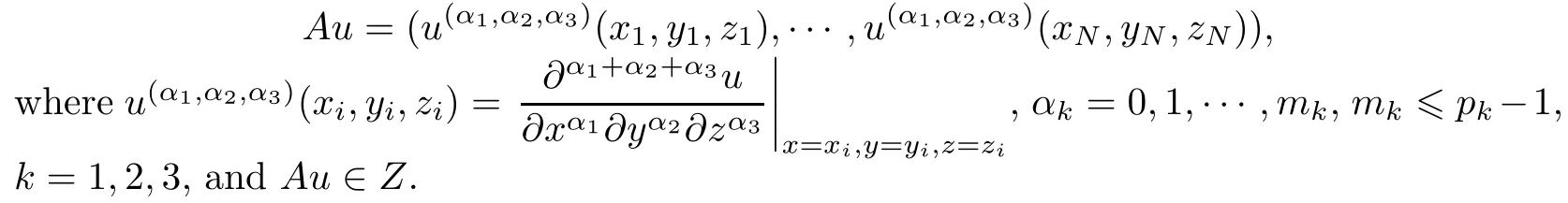
where ik=0,1,···,pk−1,k=1,2,3.Again let Z=Rrbe the r dimensional Euclidean space,A:X→Z be a linear continuous operator satisfying

Problem PFind σ(x,y,z)∈X,such that

and every cijkis a real number,then it is obvious thatusatis fies the boundary condition (2.2)and Tu=0,so u∈N(T).

On the contrary,if u∈N(T)and satis fies the boundary condition(2.2),then fromit follows that there is

3 Characterization,Existence and Uniqueness

Let N(A)={u|Au=0,u∈X}be the null space of the operatorA.For given positive integers p1,p2,p3and all u∈X,denote

Then we have the following characterization theorem.

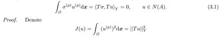
Theorem 3.1(Characterization Theorem) σ∈Xis a trivariate Hermit interpolating natural spline or the solution of the ProblemPif and only if

with u∈X and Au=z.

First,by the necessary conditions of functional minimum,if the functional J(σ+εu)get its minimum at σ,then its variation δJ=0 at σ.That is,

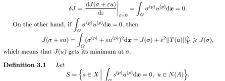
We callSthe trivariate Hermit natural spline space.

For a given z,let Az={u|Au=z,u∈X}be the collection of all functions which satis fies interpolation condition in X and assume that Az∅.Then we have

Theorem 3.2Suppose thatσ(x,y,z)is the solution of ProblemP,then for alls(x,y,z)∈Sandu(x,y,z)∈Az,one has

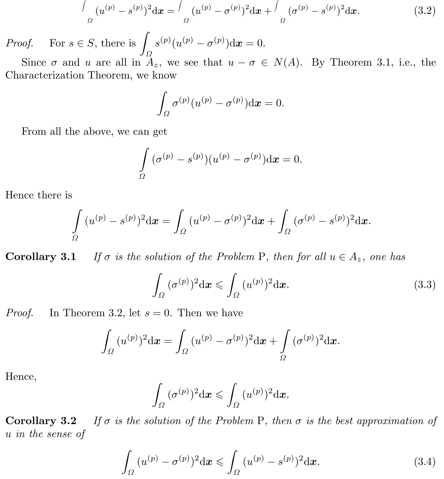
Proof.According to Theorem 3.2,it is obvious.

Corollary 3.3If the ProblemPonly has the zero solution in the spacePhp1,p2,p3iwhen the interpolating conditions are homogeneous,then the solution of the ProblemPis unique. Proof.Suppose that the Problem P have two solutions σ and˜σ.Substituting σ for u andfor s in Theorem 3.2,we get immediately

is closed in Y(see[17]).Moreover,by Theorem 2.1,the null space N(T)=Php1,p2,p3i of T is of finite dimension.From all above we know that the subspace

with the natural boundary conditions(2.2)is closed in Y(see[17]).LetΘYbe the null vector of Y.Obviously,it belongs to TN(A).If we fi x an element u∗∈Az,then it is easy to know that

Hence,TAzis closed.For the Problem P,we can consider it as a variation problem which minimizes the distance betweenΘYand TAz.Since TAzis closed,the solution of the variation problem or the Problem P exists.In other words,trivariate Hermit interpolating natural spline σ(x,y,z)does always exist.

4 Construction

Denote by N(A)⊥the orthogonal complement of N(A)in X.Using the same methods as in [11],the following Lemma 4.1 can be proved easily.

Lemma 4.1LetA∗be the conjugate operator ofA,andR(A∗)the rang ofA∗.ThenR(A∗)is anrdimensional space;moreover,N(A)⊥is also anrdimensional space.

This completes the proof.

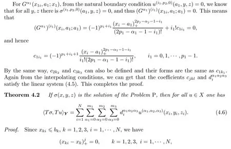
We design x=x1,y=x2,z=x3,xi=x1i,yi=x2i,zi=x3i,i=1,···,N.Then we have the following theorem.

Theorem 4.1(Construction Theorem)Trivariate Hermit interpolating natural splineσ(x,y,z)for scattered data of3Dhas explicit and compact expression as follows:

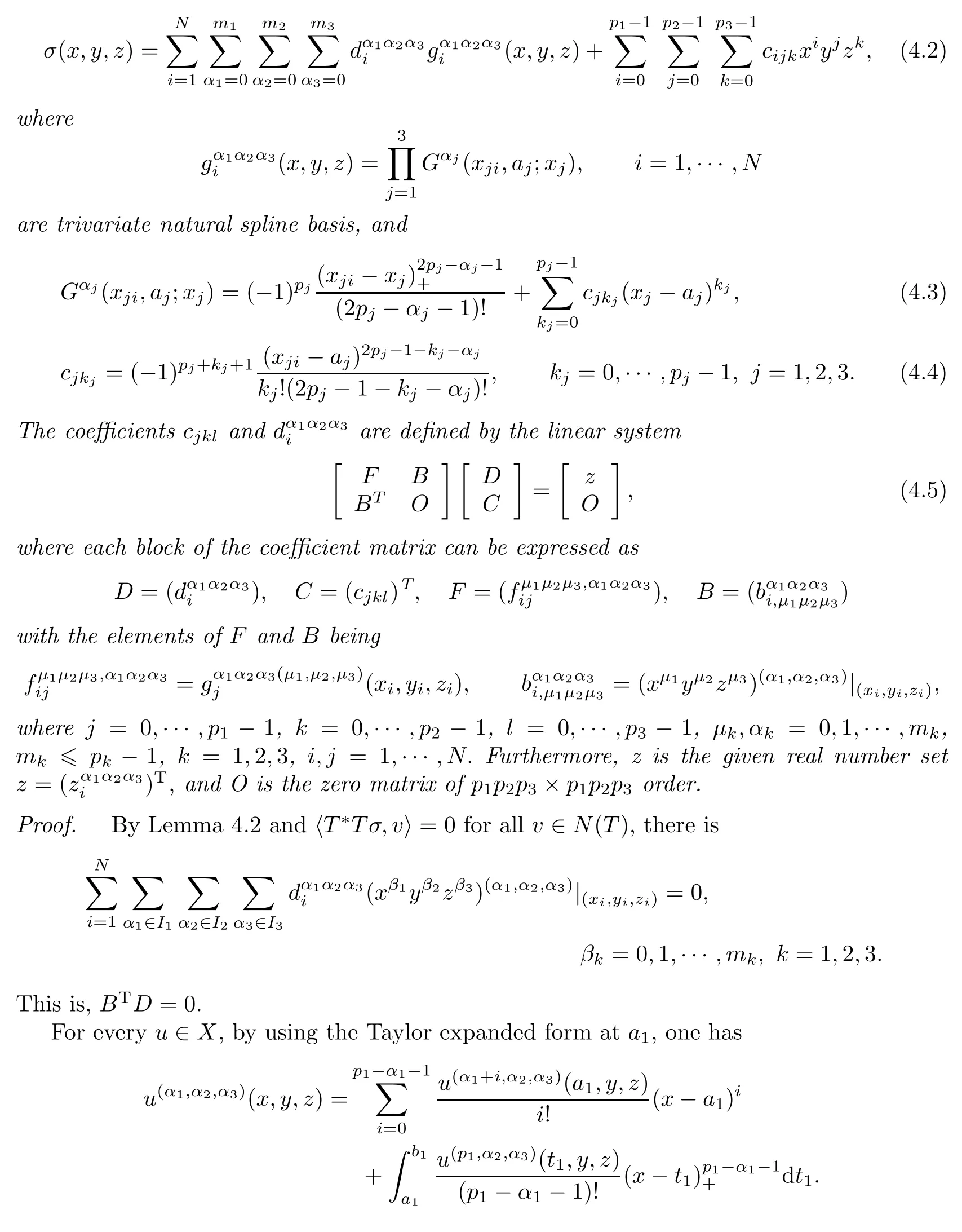
where j is any nonnegative integer.Then,doing partial integration,from BTD=0 in the proof of Theorem 4.1,we can get

Theorem 4.3The matrix of the linear system(4.5)of simple trivariate natural spline interpolation for scattered data of3D is symmetry.

Proof.Obviously,it suffices to prove that the matrix Q is symmetry.To do this,let

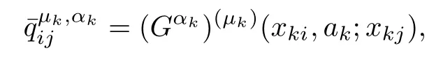
whereµk,αk=0,1,···,mk,mk6 pk−1,k=1,2,3,i=1,2,···,N,j=1,2,···,N.

Without loss of generality,assume that xki>xkj.Then

Hence,the elements of the matrix F satisfy

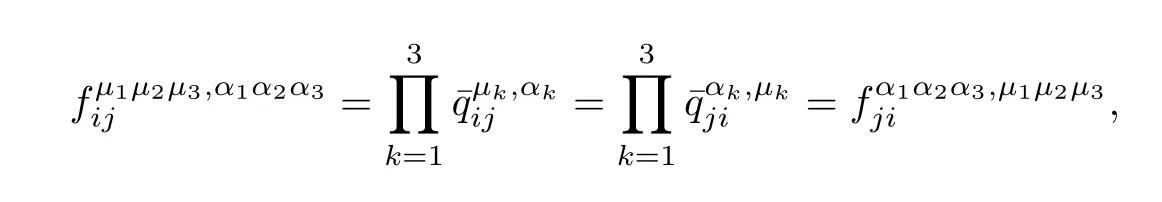
which means that F is a symmetry matrix.

Theorem 4.4IfBTD=0(D0),then the coefficient matrix of the linear system(4.5)is positive semi-de finite.

Then take σ=u=η in Theorem 4.2.By a simple computation,there is

By hTη,TηiY>0,we know DTFD>0.Thus from the arbitrariness of D and C,it is easy to know that the coefficient matrix J is positive semi-de finite.This completes the proof.

5 Numeral Examples

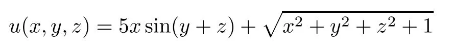
Example 5.1Take

andΩ=[0.5,4]×[0.5,4]×[0.5,4].Interpolatory points(scattered data),which are produced by random functions,belong to[1.5,3]×[1.5,3]×[1.5,3].Using h4,4,6i order Hermit natural spline interpolation function to fi t the functionuin simple case.We present the cases for 500 and 3000 scattered data points as z=2.6.The interpolatory results are listed in Table 5.1. The order of Figures 5.1 and 5.2 is scattered data,interpolatory surface and error surface.

Table 5.1 The error for z=2.6

Fig.5.1 500 scattered data

Fig.5.2 3000 scattered data

Example 5.2Take

andΩ=[−1,2]×[−1,2]×[−1,1.5].Interpolatory points(scattered data),which are produced by random functions,belong to[0,1]×[0,1]×[0,0.5].Using h4,4,4i order natural spline interpolation function σ to fi t the functionuwith Hermit interpolating conditions:

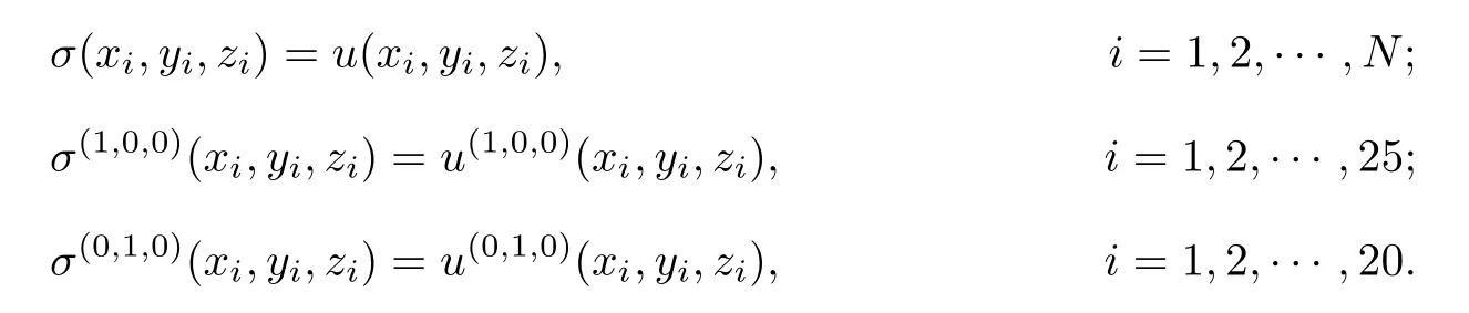
We present the cases for 300,500,1000,2000,3000 and 4000 scattered data points as z=0.3.The results are listed in Table 5.2.The order of Figures 5.3–5.8 is scattered data, interpolatory surface and error surface.

Table 5.2 The error for z=0.3

Fig.5.3 300 scattered data

Fig.5.4 500 scattered data

Fig.5.5 1000 scattered data

Fig.5.6 2000 scattered data

Fig.5.7 3000 scattered data

Fig.5.8 4000 scattered data

6 Conclusions

In this paper,we construct a new kind of trivariate Hermit natural spline to deal with the scattered data fi tting of 3D.We also study the existence,uniqueness,characterization of the solution.As we can see from the process of its construction,the new trivariate Hermit natural spline possesses the following favorite properties:

(a)Need not constructing triangulation or any other multivariate simplex meshes,without using the reproducing kernel in the Hilbert spaces,it can be constructed by a simple way and has compact and explicit expression;

(b)It is a piecewise polynomial and is a polynomial of 2pi−1 degree with respect to the variate xi,i=1,2,3.Furthermore,it can be constructed as a polynomial of different degree with respect to different variates,for example,we can do it as a polynomial of one degree for x,a polynomial of three degree for y and a polynomial of fi ve degree for z;

(c)It is not a tensor product by un-variate polynomial.

If we regard the variable z as time parameter t,then the tri-cubic natural spline can be showed by the way of 3D animation.But in this paper,we cannot do this,so we present the images of functions of two variables which come from fi xing some z in the numerical examples.From results in the numerical examples,we can find that the maximal error is mainly distributed on the boundary of the domain.

[1]Tang Z S.Visualization of 3D Data Sets(in Chinese).Beijing:Tsinghua Univ.Press,1999.

[2]Amidror I.Scattered data interpolation methods for electronic imaging systems:A survey.J. Electron.Imaging,2002,11(2):157–176.

[3]Lai M J,Schumaker L L.Spline Functions Over Triangulations.London:Cambridge Univ. Press,2007.

[4]Baraniuk R,Cohen A,Wagner R.Approximation and compression of scattered data by meshless multiscale decompositions.Appl.Comput.Harmon.Anal.,2008,25:133–147.

[5]Lai M J.Multivarariate Splines for Data Fitting and Approximation.In:Neamtu M,Schumaker L L.Approximation Theory XII:San Antonio.Brentwood:Nashboro Press,2008.

[6]Kersey S,Lai M J.Convergence of local variational spline interpolation.J.Math.Anal.Appl., 2008,341:398–415.

[7]Zhou T H,Han D F,Lai M J.Energy minimization method for scattered data hermit interpolation.Appl.Numer.Math.,2008,58:646–659.

[8]Johnsona M J,Shen Z,Xu Y.Scattered data reconstruction by regularization in B-spline and associated wavelet spaces,J.Approx.Theory,2009,159:197–223.

[9]Chen G,Lai M J.Wavelets and Spline.Brentwood:Nashboro Press,2006.

[10]Wu Z M.Models,Methods and Theories for Scattered Data Fitting(in Chinese).Beijing: Science Press,2007.

[11]Laurent P J.Approximation et Optimization.Paris:Hermann,1972.

[12]Li Y S,Guan L T.Bivariate polynomial natural spline interpolation to scattered data.J. Comput.Math.,1990,8(2):135–146.

[13]Chui C K,Guan L T.Multivariate Polynomial Natural Spline for Interpolation of Scattered Data and Other Applications.In:Conte A,et al.Workship on Comurtational Geometry.World Scienti fi c,1993:77–98.

[14]Guan L T.A Local Basis for Bivariate Polynomial Natural Splines of Scattered Data. Guangzhou International Symposium of Computational Mathematics,Guangzhou,1997:17–24.

[15]Guan L T.Bivariate polynomial natural spline interpolation algorithms with local basis for scattered data.J.Comput.Anal.Appl.,2003,2(1):77–101.

[16]Guan L T,Liu B.Surface design by natural splines over re fi ned grid points.J.Comput.Appl. Math.,2004,163(1):107–115.

[17]Bezhaev A Y,Vasilenko V A.Variational Theory of Splines.New York:Kluwer Academic/Plenum Publishers,2001.

[18]Guan L T,Xu W Z,Zhu Q Y.Interpolation for space scattered data by bicubic polynomial natural splines.Acta Sci.Natur.Univ.Sunyatseni,2008,47(5):1–4.

[19]Xu Y Y,Guan L T,Xu W Z.Trivariate odd degree polynomial natural spline interpolation for scattered data,Math.Numer.Sinica.,2011,33(1):37–47.

Communicated by Ma Fu-ming

41A15,65D07,65D17

A

1674-5647(2012)02-0159-14

date:Jan.19,2010.

Ph.D.Programs Foundation(200805581022)of Ministry of Education of China.