LI Wen-bai(李闻白)，LIU Ming-yong(刘明雍)，LIU Fu-qiang(刘富樯)，XU Fei(徐飞)

(School of Marine Engineering，Northwestern Polytechnical University，Xi’an 710072 Shaanxi，China)

Introduction

The absence of GPS underwater makes navigation for autonomous underwater vehicle(AUV)difficult，especially for offshore engineering，pipeline maintenance，environment survey and mineral resources prospect.Instead of realizing many missions with a single AUV，the future trend is to implement one mission with a fleet of AUVs［1－3］.

Among several traditional positioning and navigation methods，such as LBL，SBL，USBL etc.，long baseline navigation systems have commonly been used for positioning of underwater equipment and manned submarines，and for navigation of AUVs currently.They can offer good localization accuracy，however，some shortcomings can not be ignored，such as the time consume and high cost for deployment and the recovery of the transponders，and the repeat processes for the moved array.

Under this motivation，a new approach for multiple AUVs navigation using a single leader is presented by P Baccou et al.［4－6］in recent years.It deals with a positioning algorithm for several vehicles with respect to a leader vehicle.Its advantages are the small number of sensors and the independence towards a beacon network.However，since it is not possible to determine the vehicle’s position from single distance information，the follower vehicle has to maneuver properly relative to the leader to provide sufficient solving conditions.This extra process increases the complexity of the navigation system，and the real-time property as well as the robustness for the system decrease somewhat.

Aiming to solve the problem above，in this paper，a robust navigation method for multiple AUVs is proposed on the basis of motion radius vectors(MRV)estimation.It is used to determine the relative positions of the members in the AUV group，as shown in Fig.1.The position information can be shared by each individual AUV through acoustic communications. Then，combined with the dead reckoning data，the positioning problem for each AUV can be solved by using a recursive trigonometry technique and an extended Kalman filter(EKF).It needs not to deploy beacons，and is not limited by the fields of action，and the vehicles can be located anywhere in a frame defined by the leader without any external transponder.Furthermore，it does not rely on the existence of high performance Doppler inertial navigation systems，only a basic dead reckoning capability is sufficient.Also，the positioning algorithm is objective and concise，therefore the navigation system is easy to be real-time and robust.

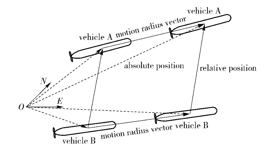
Fig.1 Motion radius vectors and vehicles’relative positions

1 Mathematical Model

The master and slave vehicles will be equipped with individual navigation systems.Each of them consists of a magnetic compass and a Doppler velocimeter to provide information necessary for dead reckoning，and an acoustic modem to implement communication.

Some notations and assumptions are introduced first.

1)Both AUVs A and B can determine the distance between them rAB()at time，where k denotes kth data transfer between A and B.

2)A and B exchange their individual dead reckoning data also at time.The position estimation of vehicle A’s own dead reckoning navigation system at timecan be denoted by()=［()()］T.

The key for the solution of the cooperative navigation problem is to know the consecutive distances and motion radius vectors between two vehicles，as shown in Fig.2.A set of distances can be generated from the real measurements which geometrically determine the relative position of vehicle B to vehicle A uniquely by a trigonometry technique.It can be seen from Fig.2 that these distances are the range observations of three consecutive modem connections，，，the MRVs，for vehicle A and MRVs，for vehicle B，taken at consecutive time instances of connection between A and B.It should be noticed that，although the individual position estimations of the dead reckoning navigation systems of A and B have drift errors，the MRVs of each vehicle will relatively be precise，depending on the quality of the dead reckoning sensors and on the time interval taken for MRVs.

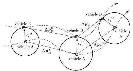
Fig.2 Relative distances and MRVs between master and slave AUVs in consecutive interval

Assuming that the measurements of the relative distances at a certain moment areand the MRVs arewe have the following relations

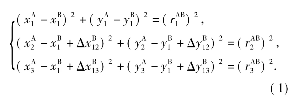
Since the AUV’s depth data can be precisely measured by a pressure sensor，we can assume that vehicle A and vehicle B have the same depth for simple presentation.Without loss of generality，let vehicle A be the leader having its own correct position.Then，the unknown position coordinates(xB1，yB1)of the follower B can be found from Eq.(1).The updated positions of vehicle B can then be obtained by adding the appropriate MRVs.Eq.(1)defines a set of algebraic equations.A necessary condition for the existence of its unique solution is that the three vectorsare linearly independent.That is，the vehicles A and B should not move on parallel straight lines with the same speed.Otherwise，the cooperative positioning problem can not be solved.It coincides with intuition，and the navigation system is unobservable under this condition.

In practice，we will avoid solving Eq.(1)directly by an algebraic or numeric algorithm，since an exact solution might show large sensitivity with respect to the input data，especially nearby the unobservable condition.Therefore，an EKF algorithm is adopted in this paper.

2 Cooperative Navigation Algorithm

2.1 Relative Position Estimation

The state vector of the system can be defined as the relative position=pB－pAand its first derivative vAB.Moreover，letrepresent the relative position of vehicle A and B at timeof the last data transfer between the modems of two vehicles.Then，the state equation of the navigation system can be written as

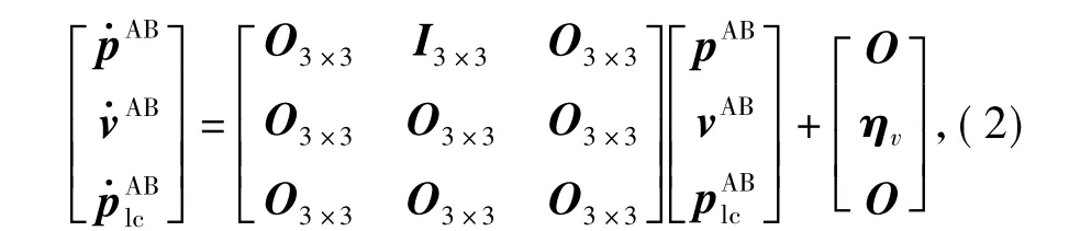
where ηvis a Gaussian noise with covariance var ηv=diag{，，0}.Eq.(2)describes the prediction of the relative position vector pABbetween two modem connection of A and B.The motivation of this model is to express the MRVs incrementsas functions of the state of system(2).

In practice，the above model is assumed to be updated with a time increment Ttu.Then，the time discrete prediction equations are

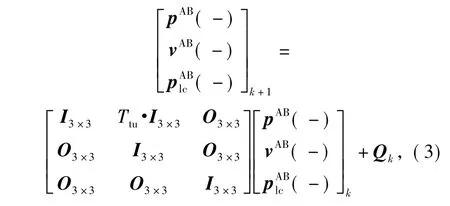
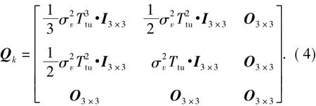
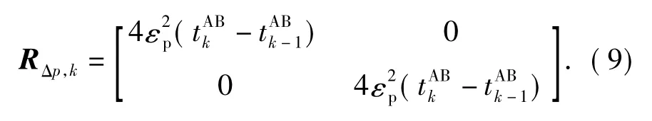
where the time discrete process noise matrix Qkobtained from Eq.(2)is

2.2 Measurement Data Update

The master AUV A can periodically receive position updates from the dead reckoning navigation of the slave AUV B.Moreover，AUV A gets position updates from its own navigation system nearly continuously in time.Based on our assumptions，the position data known by master vehicle A has the property that the position errors will not be bounded over time.They will show a characteristic drift with a bound increasing with time，and depend on the quality of the sensors used.Therefore，a proper noise model to describe the position error is the integrated white Gaussian noise model，

The crucial step in the cooperative navigation algorithm is the following observation equation related to MRV

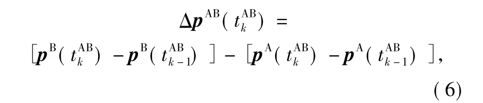
i.e.，the difference vectors of two consecutive position observations of vehicle B relative to vehicle A.Combined the dead reckoning information and Eq.(5)，we obtain the error distribution of the position difference observations

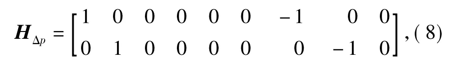
Then，the position difference measurement matrix can be written as

and the associated measurement noise matrix is

Let Pk(－)be a priori covariance estimate at tAkB.Suppose that a new observation ΔpAkBis available for A via the communication module.Then，two substitutions have to be made to realize covariance update.Firstly，the state describing the relative position at last connection has to be rewritten as

and let it represent the current estimate of the relative position.Secondly，the covariance matrix which describes the cross correlation between(+)and ΔpAB(+)has to be updated according to

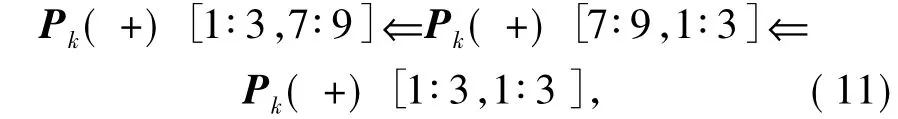
where the brackets denote the indicated sub-matrices.

2.3 Selection of Measurement Data

Before the relative position measurements can be processed by EKF，it is important to discard the bad relative position measurements to keep the filter stable.In order to decide if a measurement pAB()obtained atis good，the state estimation error covariance matrix Pk(－)can be used.Its diagonal terms are variances of errors in estimates of the state variables.For the state vector sthe first two terms on the principal diagonal of Pk(－) are the variancesandof the errors in the estimates of relative positionandrespectively.Using these variances，a circular region of position uncertainty around the relative position estimate atwith radius

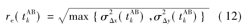
can be defined.Given the relative position estimate at，the expected measurement is

A measurement pAB()is good，if it satisfies

Any measurement pAB()that does not satisfy Eq.(14)should be discarded.

3 Observability Analysis

The observability refers to computability of the state of a dynamic system from measured data.That is，this inversion problem can be solved without knowing a priori knowledge about the state variables［7－8］.From the above discussion，we know that，when two vehicles go along parallel straight lines with the same speed，the navigation system is globally unobservable.Therefore，we will further explore the locally observable conditions for the system.

Consider a special case of two consecutive data transfer actions between A and B.Define the simplified measurement vector

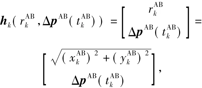
as a function of relative range rABand MRV difference ΔpAB.Then，after a sampling period

Calculated that the Jacobian determinant of the mappingh［k，k+1］，we obtain

For local observability，it is sufficient that Jh［k，k+1］does not vanish，i.e.，

Examining Eq.(16)carefully，we find that the navigation system is locally observable，if and only if two consecutive position data pAB()and pAB()are linearly independent.Therefore，Eq.(16)can be used as a criterion to check the system’s observability.Let δ0be a small positive constant.For two consecutive relative position observations pAB()and pAB()，ifsatisfy

then，the navigation system is unobservable or nearly unobservable.And，the motion trajectory of the vehicles should be readjusted to keep the system observable.

4 Simulation Results

Simulation results obtained by a typical area searching mission that is important for ocean exploration are presented to verify the effectiveness of the proposed cooperative navigation algorithm.In this mission，the leader，vehicle A，navigates along an“M”trajectory ABCDE and the follower，vehicle B，navigates along A1B1C1D1E1，as shown in Fig.3.

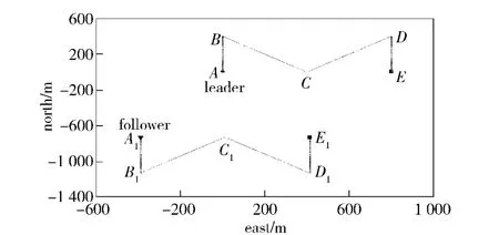
Fig.3 Area searching mission

The initial positions of vehicle A and vehicle B are about(0 m，0 m)and(－700 m，－400 m)respectively. Then， in the cooperative navigation process，the sensors’sampling period is 0.2 s，the EKF update time increment is Ttu=1 s.The velocity of vehicles is 1 m/s with(0.05 m/s)2，the heading is measured by a compass with=(0.5°)2，and the measurement noise of relative range is=(0.1 m)2.All the measurement noises are Gaussian with zero mean.

Figure 4 shows the statistical averages of the follower vehicle’s positioning error，which is obtained by using Monte Carlo method in 100 repeated simulations.It can be seen from Fig.4 that the dead reckoned positioning error fluctuates remarkably when vehicle B turns.This is caused by the mismatch between the kinematic model of the vehicle and the actual vehicle dynamics in turning maneuvers［9－10］.In comparison，the positioning errors of vehicle B estimated by vehicle A using EKF is more stable，although there are still some fluctuation in turning maneuvers.This is due to the accurate relative position observations provided by vehicle A and the testing condition(14)，which largely prevents the bad measurements，for instance，the data collected in vehicle turning，to undermine the performance of the filter.In the entire course，the positioning error of our navigation method is less than 3 m，and it seems to offer some robustness with respect to mismatching of the vehicle maneuvers.

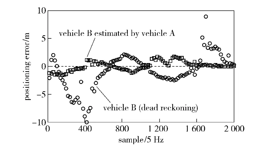
Fig.4 Positioning error of vehicle B

Next，we further analyze the real-time property of the cooperative navigation algorithm.Table 1 shows the CPU computation time，in the simulation time of 2 000 s，of two navigation algorithms presented in this paper and in Ref.［4］respectively under the same initial conditions.

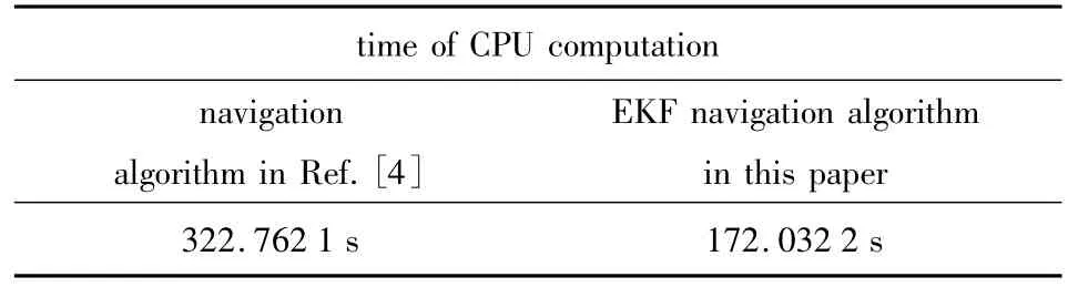
Table 1 Time of CPU computation

From Table 1，it can be seen that the CPU computation time for our navigation algorithm is only about 53.3%of the algorithm in Ref.［4］.Therefore，the navigation algorithm in this paper is more efficient and has better real-time property.

5 Conclusions

This paper presents a cooperative navigation algorithm for a group of autonomous underwater vehicles based on motion radius vectors estimation.It is shown that the relative positioning problem is solvable when the dead reckoning data and relative position are shared by AUV members through an acoustic communication network.A novel approach for solving the relative positioning problem is proposed，which is achieved by a recursive trigonometry technique and EKF.The simulation results show that this navigation method has good positioning accuracy and real-time property，and it is robust with respect to mismatching of the vehicle maneuvers.

［1］Kinsey J，Eustice R，Whitcomb L.A survey of underwater vehicle navigation:recent advances and new challenges［C］∥Proceedings of the IFAC Conference of Manoeuvering and Control of Marine Craft，Lisbon Portugal 2006:1－12.

［2］Chanderasekhar V，Winston S，Yoo C，How E.Localization in underwater sensor networks-survey and challenges［C］∥Proceedings of the 1st ACM International Workshop on Underwater Networks，New York，2006:33 －40.

［3］Stutters L，LIU H，Tiltman C，Brown J.Navigation technologies for autonomous underwater vehicles［J］.IEEE Transactions on Systems，Man and Cybernetics，Part C:Applications and Reviews，2008，38(2):581 －589.

［4］Baccou P，Jouvencel B.Simulation results，post-processing experimentation and comparison results for navigation，homing and multiple vehicle operations with a new positioning method using a transponder［C］∥Proceedings of the 2003 IEEE/RSJ International Conference on Intelligent Robotics and Systems，Las Vegas，2003:811 －817.

［5］Baccou P，Jouvencel B，Creuze V.Single beacon acoustic for AUV navigation［C］∥Proceedings of International Conference on Advanced Robotics，Budapest，Hungary，2001:22－25.

［6］Vaganay J，Baccou P，Jouvencel B.Homing by acoustic ranging to a single beacon［C］∥Proceedings of Oceans 2000 MTS/IEEE，Conference on Exhibition，Providence，2000:1457－1462.

［7］Gadre A，Stilwell D.Toward underwater navigation based on range measurements from a single localization［C］∥Proceedings of IEEE International Conference on Robotics and Automation，New Orleans，2004:1－6.

［8］Gadre A，Stilwell D.Underwater navigation in the presence of unknown currents based on range measurements from a single localization［C］∥Proceedings of American Control Conference，Portland，2005:1816－1821.

［9］Engel R，Kalwa J.Coordinated navigation of multiple underwater vehicles［C］∥Proceedings of the 7th International Offshore and Polar Engineering Conference，Lisbon，Portugal，2007:1 －8.

［10］Engel R，Kalwa J.Relative positioning of multiple underwater vehicles in the grex project［C］∥Proceedings of Oceans 2009 MTS/IEEE，Conference on Exhibition，Bremen，Germany，2009:1－7.