S.Saravanan，F.Ju，N.Q.Guo

（1.School of Mechanical ＆Aerospace Engineering，Nanyang Technological University，Singapore；2.School of Engineering，Monash University，Bandar Sunway 46150，Selangor，Malaysia）

1 Introduction

Composite materials are widely and increasingly used due to their low weight，high specific stiffness and strength，good fatigue performance and excellent corrosion resistance. The major disadvantage of composite structures is the high probability of severe degrading of mechanical properties in the presence of damage especially in the through－thickness direction.The unique anisotropic，low－conductivity and low－permeability characteristics of composite materials have limited the applications of traditional nondestructive evaluation（NDE）techniques in damage detection.In addition，traditional NDE testing is usually timeconsuming point testing thus not suitable for large structure inspection.

The long－range damage detection potential of Lamb waves has been studied extensively1－9.The interaction between Lamb wave and damage will modify the response wave signal from which information related to damage can be extracted for automated damage detection. However， the interpretation of the response wave signal is not easy due to the complex nature of the wave－damage interaction.

Artificial neural network（ANN）is a powerful computational tool for pattern recognition and function approximation and has been tried in Lamb wave－based damage detection10，11.However，the accuracy of the network has been limited by the redundant highdimensional features and the very complicated network architecture.In this paper，a new damage detection scheme is proposed which uses signal demodulation for feature extraction，an unsupervised neural network for clustering and feature dimensionality reduction，and a supervised neural network for damage characterization.

2 Numerical simulation of lamb waves

2.1 Numerical model for simulation

A 2D unidirectional composite laminate with a notch defect is modeled for simulation.The laminate is 300mm long and 1mm thick as shown in Figure 1.The notch is located at x mm from the left end of the laminate with width 0.4 mm and depth y mm.The element size is 0.2mm×0.125mm，and the time step is 0.011 099 9μs.

Figure 1.A 2Dnumerical model of a unidirectional composite laminate

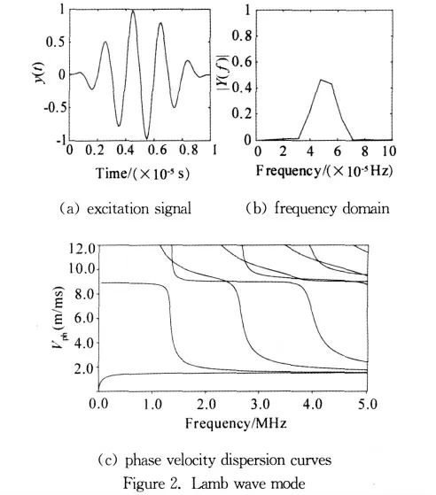
A five－cycle sinusoidal signal modulated by a hanning window with the center frequency of 500kHz is applied at the left end in the x－direction in the form of pressure to excite S0Lamb wave mode，as shown in Figure 2.The phase velocity dispersion curve for S0in Figure 2 is quite flat at the chosen operation frequency.

2.2 Damage cases

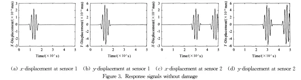
Thex－andy－displacement response signals at sensing point 1（75mm）and 2（225mm）in Figure 1 are recorded during simulation.A simulation without damage is performed first and the results are plotted in Figure 3.Then simulations are performed for 21notch locations（x：100－200mm，Δx：5mm）and 7notch depths（y：0.125～0.875mm，Δy：0.125mm），the combination of them results in 147damage cases in total.For example，the response signals when the notch is at the middle（x＝150mm andy＝0.5mm）are plotted in Figure 4.By comparing with Figure 3，there are additional wave packets and change of amplitude due to wave－damage interaction such as reflection，diffraction and mode conversion.So the response signals contain the information associated with damage state from which features can be extracted for damage characterization.

3 Feature extraction

3.1 Baseline subtraction

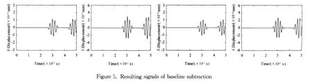
The signals in Figure 3are used as the baselines and subtracted from the signals in Figure 4thus the resulting signals indicate the effect of damage on the response signals，as shown in Figure 5.

3.2 Wave signal demodulation

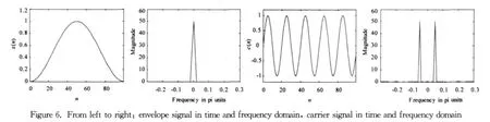
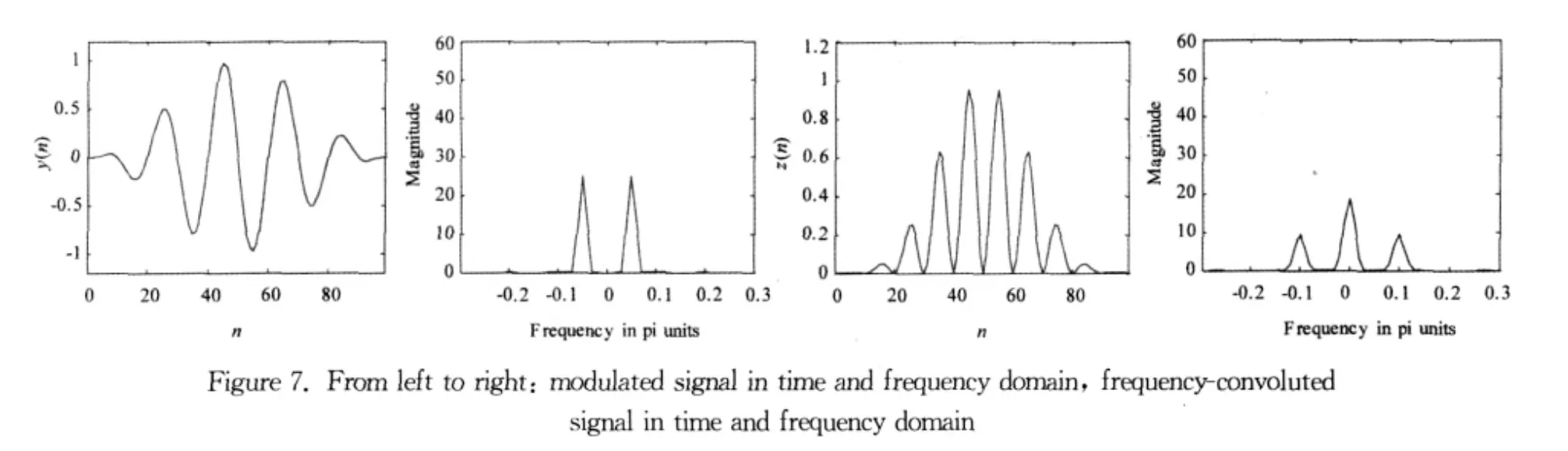
Each wave packet in Figure 5can be considered as a low－frequency envelope signalx（n）modulated by a high－frequency sine carrier signalc（n）as shown in Figure 6.The modulation operation is carried out by multiplication in the time domainy（n）＝x（n）·c（n），which results in the convolution in the frequency domainY（ω）＝X（ω）＊C（ω），as shown in Figure 7.The modulated signal is then transmitted through the plate and received by the sensor.In order to retrieve the envelope signal from the received signal，the received signal is convoluted by itself in the frequency domainZ（ω）＝Y（ω）＊Y（ω）as shown in Figure 7.It is obvious that the resulting signalz（n）has a lowfrequency component and a high－frequency component in 0≤ω≤π／2 which can be separated by a lowpass filter with the cutoff frequency in between.The magnitude response of the filter is shown in Figure 8 and the system function is：

The signalz（n）is then filtered with this lowpass filter and the result is shown in Figure 8，which is a slightly delayed envelope signal.This demodulation algorithm for envelope extraction is computationally more efficient than the conventional Hilbert transform and do not have discrepancies at two ends.

3.3 Peak extraction

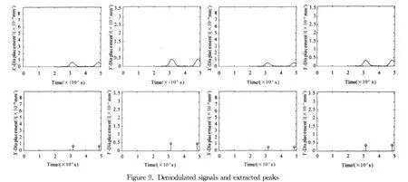
The signals in Figure 5are demodulated with the above algorithm and the results are shown in Figure 9，which are related to the energy change due to the wave－damage interaction. The peak values and locations are extracted by finding the local maxima and combined into the following 8－dimensional feature vector：

wherepkixandpkiyare the peak values at sensor i in thex－andy－direction，respectively.locixandlociyare the peak locations at sensor i in thex－andydirection，respectively.The feature vectors will be used as input vectors to the unsupervised and supervised artificial neural networks for pattern recognition.

4 Unsupervised learning（SOM）

4.1 SOM neural network

The self－organizing map （SOM）12is an unsupervised artificial neural network model for nonlinearly mapping the high－dimensional input vectors onto a low－dimensional，topologically ordered array of neurons，inspired by the topographical mapping ability of the human brain cortex.It has become a powerful tool for clustering，feature selection and highdimensional data visualization due to its properties of input space approximation，topological ordering and density matching13.In this paper，a two－dimensional 4×4Kohonen SOM neural network is used and the architecture is shown in Figure 10.

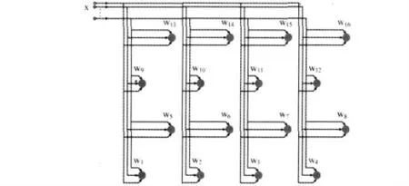
Figure 10.The architecture of the SOM neural network

The training of the SOM is based on unsupervised competitive learning consisting of five essential processes：

（1）Initialization.The initial synaptic weight vectorswj（0）of neurons are first assigned small random values which should be different from each other.

（2）Competition.A discriminant function related to the distance between the input vectorxand the weight vectorwjis selected and its value is calculated for each neuron in the network.The neuroni（x）with the minimum discriminant function value is called the winning neuron：

where‖·‖is the Euclidean norm，andi（x）is the index of the winning neuron.

（3）Cooperation.A topological neighborhoodhj，iof cooperating neurons centered on the winning neuron is determined with the following Gaussian topological neighborhood function：

wheredj，iis the lateral distance between winning neuroniand cooperating neuronj，σ（n）is the width of the Gaussian function with initial valueσ0and time constantτ1，nis the number of iterations.

（4）Weights adaptation.The synaptic weight vectors of all neurons are updated using the following equations：

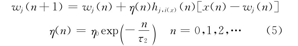
whereη（n）is the learning rate with initial valueη0and time constantτ2.

（5）Iteration.Repeat processes（2）～（4）by randomly presenting the training samples to the network until the stopping criterion is met，which can be the predefined number of iterations or the small rate of changes in the map's weights.

4.2 Damage clustering using SOM

An important ability of the SOM neural network is clustering the data into different categories in an unsupervised manner.For example，the peak values of all samples are used as 4－dimensional input patterns to the SOM network in Figure 10.After training without the damage information，the network converges and 7 clusters are formed with 11samples in each，as shown in Figure 11.By checking the samples in each cluster，it is found that samples with the same severity of damage（depth of the notch）are sorted into the same cluster.Now the clusters can be labeled with damage level 1－7.If a new input pattern with unknown damage severity is presented to the SOM，it will be sorted into the cluster which is most activated and the damage severity can be estimated from the cluster label.Similarly，if the peak locations of all samples are used as input patterns to the SOM network，11 clusters are formed with 7samples in each，as shown in Figure 11.It is observed that samples with the same damage location are clustered together.

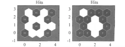
Figure 11.Clusters formed by the SOM neural network

4.3 Feature dimensionality reduction using SOM

Another important application of the SOM neural network in pattern recognition is the dimensionality reduction of features. This can save a lot of computational cost in the damage detection algorithm if the features are high－dimensional and correlated.Although dimensionality reduction can also be achieved using traditional principal component analysis（PCA）14，the SOM is more advantageous in visualization and will not lose the real meaning of features.In order to reduce the dimensionality of the features acquired in the feature extraction session，the feature vectors of all damage cases are used as input vectors to the SOM neural network.After training and convergence of the network，the weights are plotted in the weight planes in Figure 12.The 8weight planes correspond to the 8elements of the input vector.Each element in the weight plane represents the connection（weight）between one input element and one neuron，with the darkness of color indicating the magnitude of the weight.If the weight planes of two input elements are very similar，the two input elements are highly correlated.It is observed from Figure 12that the weight plane 1，3，5，7are almost the same，this means the input element 1，3，5，7are correlated.Also the correlation between input element 2and 4can be found from weight plane 2and 4.Therefore，the dimensionality of the 8－dimensional feature vector in Equation （2）can be reduced by eliminating the correlated elements，resulting in the following 4－dimensional feature vector which will be used as input to the supervised neural network：

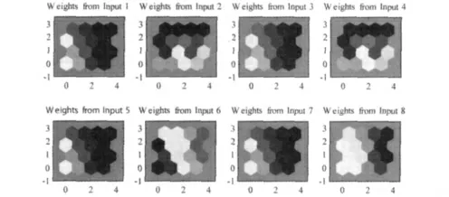
Figure 12.Weight planes of the SOM neural network

5 Supervised learning（MLP）

5.1 MLP neural network and BP learning algorithm

The multi－layer perceptron（MLP）neural network is the most widely used model of supervised neural network due to its excellent performance in function approximation， associative memory and pattern classification.The typical MLP neural network is a feed－forward network containing one input layer，one or more hidden layers and one output layer，as shown in Figure 13.The input layer neurons do not perform any computation and just distribute the input vectors to the hidden layer.The hidden layer and output layer neurons are computational neurons with a continuously differentiable nonlinear activation functionφ（·），which can be sigmoidal functions such as the following logistic or hyperbolic tangent function：

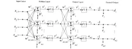
Figure 13.The architecture of the MLP neural network

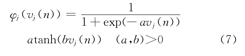
wherevj（n）＝（n）is the activation signal of neuronjat iterationn.

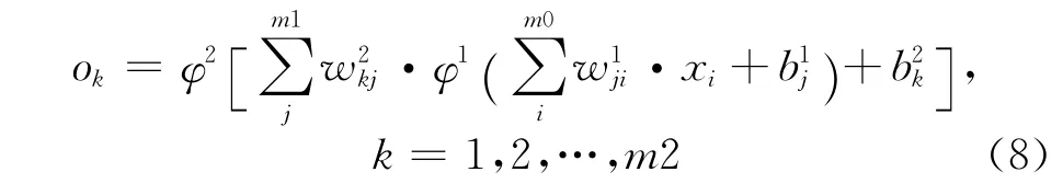
The training of the MLP neural network is in a supervised manner.During the training process，the input vectorxis presented to the network and the outputois generated by the network.By comparing the output with the a priori desired outputd，an error signale＝d－ocan be obtained.Then the adjustments to the synaptic weights of the network are calculated based on the error signal so that the network output can approximate the desired output.The weight adjustments of the output layer neurons can be easily determined using optimization methods such as the gradient descent.However，the calculation of the weight adjustments of the hidden layer neurons becomes a problem which has not been solved until the development of the back－propagation （BP）algorithm15.This algorithm has become the most popular learning algorithm for the training of MLPs due to its high computational efficiency.In the BP algorithm，two passes of computation are identified13：the forward pass and the backward pass.In the forward pass when the synaptic weights remain unchanged，the function signals come in at the input layer，propagate forward on a neuron－by－neuron，layer－by－layer basis and emerge at the output layer as output signals in Equation（8）：

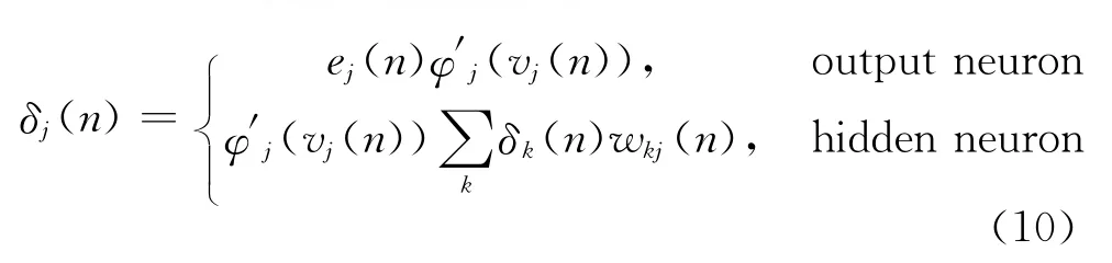
In the backward pass，the error signals are computed at the output layer，propagate backward，layer－by－layer， accompanied by the recursive calculation of the local gradient for each neuron which enables the adjustment of synaptic weight in the following delta rule：

whereΔwji（n）is the correction applied to the synaptic weight connecting neuronito neuronj，ηis the learning rate，δj（n）is the local gradient，andyi（n）is the input signal of neuronj.The calculation of the local gradient is shown in Equation （10），depending on whether neuronjis an output or a hidden neuron：

The training process is iteratively performed by presenting epochs of training samples to the network until the stopping criterion is met，which can be the predefined number of iterations or the small rate of change in the mean square error.

5.1 Damage characterization using MLP

According to the universal approximation theorem16，any continuous nonlinear function with a finite number of discontinuities can be approximated arbitrarily well by a MLP neural network having one hidden layer of sufficient neurons.In this paper，a MLP neural network is used to approximate the unknown inverse model of the structure in order to estimate the notch parameters providing the features extracted from the response signals.The network has the architecture shown in Figure 13 with one input layer ofm0neurons，one hidden layer ofm1neurons and one output layer ofm2neurons.Herem0＝4（number of dimensions of the input vector）andm2＝2（number of notch parameters to be estimated）.The number of hidden neuronsm1 which governs the express power of the network depends on the complexity of the function to be approximated.According to the Ockham's razor principle，the simplest network which can adequately fit the training set is more preferred.Unless special conditions of the problem are given，a three－layer network（one hidden layer）is sufficient to approximate any arbitrary function.Complex network with more hidden layers and neurons are more susceptible to overfitting which leads to poor generalization.Therefore only 6hidden neurons are used in this paper and this simple network performs well.

The number of training samples should be more than the number of weights in the network.A rule of thumb for determining the number of training samples is14：

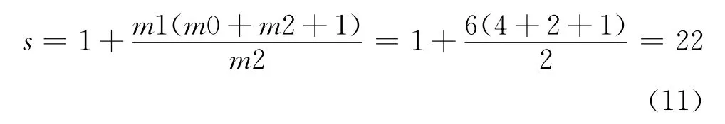
Since there are 147damage cases，the training samples are enough.

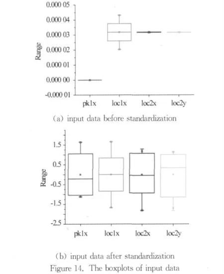
The elements in the feature vector extracted from the response signal have different orders of magnitude.If they are directly presented to the network for training，the elements with higher orders of magnitude will have dominant effect on the weight adjustments.In order to avoid this，standardization is performed to transform the input and target data into standardized data with zero mean and unit variance using the following equations：

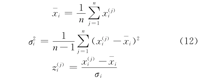
wherex（j）iis the ith element of the jth sample，is the mean，σ2iis the variance，andz（j）iis the standardized data.The boxplots of input data before and after standardization are shown in Figure 14.

The standardized data set is then randomly divided into a training set and a testing set，with the ratio of 0.8to 0.2.The testing set is not used during training，but provides an independent test of the network's generalization ability.

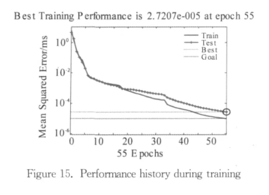
The stopping criterion is set asMSE＝1×10－5，which is the mean square error in the standardized space.After 55 epochs of training，the stopping criterion is met and the performance history of the network is plotted in Figure 15and 16.The result shows a good generalization of the network since the performance on the testing set are quite close to that on the training set.And no evidence of overfitting is observed.

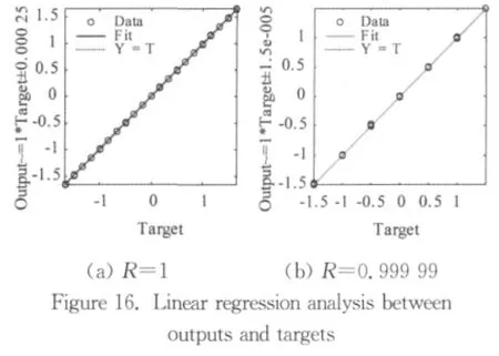
In order to further assess the performance of the network，the entire data set is presented to the trained network and a linear regression analysis is carried out between the network outputs and the corresponding targets.The result is shown in Figure 15.Since the output vector is 2－dimensional，there are two plots.Both of them show the strong linear relationship between outputs and targets，with the correlation coefficients of 1and 0.999 99respectively.This means that the network fits the entire data set well.

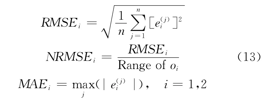
Finally，the errors between the network outputs and corresponding targets are calculated in the original space in terms of the root mean square error（RMSE），the normalized root mean square error（NRMSE）and the maximum absolute error （MAE），which are defined as follows：

And the results in Table 1show that the errors are quite small，therefore the accuracy of the trained network is reasonably high.

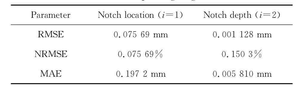
Table 1.Errors between the network outputs and corresponding targets

Now the trained network can be used to detect unknown notches by extracting feature vectors form the response signals and presenting them to the network.

6 Conclusion

A damage detection algorithm based on Lamb wave signal demodulation and ANNs has been proposed in this paper， consisting of feature extraction，clustering，feature dimensionality reduction and damage characterization.The validity of this damage detection algorithm is verified using a FE model of a composite laminate with notch defects.The wave signal demodulation algorithm is able to demodulate the response Lamb wave signal into the envelope signal and extract peaks which are related to the energy change due to damage.Then the peak values and locations are combined into an 8－dimensional feature vector which is used as the input vector to ANNs.A 4×4SOM neural network is first employed in an unsupervised manner and it is shown that this network is capable of clustering the damage cases into categories according to the damage severity or location.Feature dimensionality reduction is also performed by this network to reduce the original highly correlated 8－dimensional feature vector into a 4－dimensional one.The 4－dimensional feature vector is then used as the input to a MLP neural network with simple architecture for damage characterization.The training of this network is in a supervised manner and based on BP algorithm.The performance of this network is then assessed using an independent testing set，the regression analysis and the evaluation of errors.It is shown that this network has high accuracy and good generalization ability.The developed system and methodology will be used and tested for future experimental signals and 3Dsimulation signals.

［1］ Alleyne DN，Cawley P.The interaction of Lamb waves with defects［J］.IEEE Trans Ultrason Ferroelectr Freq Control，1992，39（3）：381－397.

［2］ Guo N，Cawley P.The interaction of Lamb waves with delaminations in composite laminates［J］.J Acoust Soc Am，1993，94（4）：2240－2246.

［3］ Guo N，Cawley P.Lamb wave－propagation in composite laminates and its relationship with acousto－ultrasonics［J］.Ndt ＆E International，1993，26（2）：75－84.

［4］ Guo NQ，Cawley P.Lamb wave reflection for the quick nondestructive evaluation of large composite laminates［J］.Mater Eval，1994，52（3）：404－411.

［5］ Alleyne D，Cawley P.The long range detection of corrosion in pipes using Lamb waves［G］.Annual Review of Progress in Quantitative Nondestructive Evaluation.Snowmass Village：Plenum Press Div Plenum Publishing，1994：2073－2080.

［6］ Scudder LP，Hutchins DA，Guo NQ.Laser－generated ultrasonic guided waves in fiber－reinforced plates －Theory and experiment［J］.Ieee Transactions on Ultrasonics Ferroelectrics and Frequency Control，1996，43（5）：870－880.

［7］ Lemistre M，Balageas D.Structural health monitoring system based on diffracted Lamb wave analysis by multiresolution processing［J］.Smart Mater Struct，2001，10（3）：504－511.

［8］ Jian XM，Guo N，Li MX，et al.Characterization of bonding quality in a multilayer structure using segment adaptive filtering ［J］. Journal of Nondestructive Evaluation，2002，21（2）：55－65.

［9］ Bartoli I，FL di Scalea，Fateh M，et al.Modeling guided wave propagation with application to the long－range defect detection in railroad tracks［J］.NDT E Int，2005，38（5）：325－334.

［10］ Su ZQ， Ye L. Lamb wave－based quantitative identification of delamination in CF／EP composite structures using artificial neural algorithm［J］.Compos Struct，2004，66（1－4）：627－637.

［11］ Lu Y，Ye L，Su ZQ，et al.Artificial Neural Network（ANN）－based Crack Identification in Aluminum Plates with Lamb Wave Signals［J］.J Intell Mater Syst Struct，2009，20（1）：39－49.

［12］ Kohonen T.The self－organizing map［J］.Proc IEEE，1990，78（9）：1464－1480.

［13］ Haykin SS. Neural networks： a comprehensive foundation，Prentice Hall，Upper Saddle River，NJ（1999）.

［14］ Zang C，Imregun M.Structural damage detection using artificial neural networks and measured FRF data reduced via principal component protection［J］.J Sound Vibr，2001，242（5）：813－827.

［15］ Rumelhart DE，Hinton GE，Williams RJ.Learning representations by back－propagating errors［J］.Nature，1986，323（6088）：533－536.

［16］ Cybenko G.Approximation by superpositions of a sigmoidal function［J］.Mathematics of Control，Signals，and Systems，1989，2（4）：303－314.