A sport and a pastime: Model design and computation in quantum many-body systems
2022-12-28GaopeiPan潘高培WeilunJiang姜伟伦andZiYangMeng孟子杨
Gaopei Pan(潘高培) Weilun Jiang(姜伟伦) and Zi Yang Meng(孟子杨)
1Beijing National Laboratory for Condensed Matter Physics and Institute of Physics,Chinese Academy of Sciences,Beijing 100190,China
2School of Physical Sciences,University of Chinese Academy of Sciences,Beijing 100049,China
3Department of Physics and HKU–UCAS Joint Institute of Theoretical and Computational Physics,The University of Hong Kong,Pokfulam Road,Hong Kong SAR,China
Keywords: quantum Monte Carlo,non-Fermi-liquid,quantum phase transition,twisted bilayer graphene
1. Introduction
In the 200 pages short novel “A Sport and a Pastime”[1]–generally regarded as a modern classic–the writer and the great stylist James Salter,has successfully established the standard not only for fiction, but for the principal organ of literature–the imagination.
Set in provincial France in the 1960s, through the wanderings of a young American middle-class college drop-out Philip Dean and an even younger, small-town French girl,Anne-Marie, the novel reveals the country’s “secret life···into which one can not penetrate”. It is “the life of photograph albums, uncles, names of dogs that have died”. The green, bourgeois and rural France would be inaccessible, remote, and lifeless to Philip Dean without his affair with the beautiful, though cheap, Anne-Marie. In a way she becomes Philip, and together they become the person who illuminates travel, the person the readers always dream of meeting, and without whom the museums are tedious,the roads empty,the rivers are dry and the food and drinks a necessity. Anne-Marie provides Dean, twenty-four and a dropout from Yale, a perspective,rescuing him from the lost ranks of student sightseers and together they provide the readers a personal reference,in which the architecture, mountains, great rivers, villages and green scenery can be easily understood from an emotional as well as numerical scale.[2]
The book,as has been praised as“what appears at first to be a short,tragic novel about a love affair in provincial France is in fact an ambitious, refractive inquiry into the nature and meaning of storytelling,and the reasons artists are compelled to invent. That such a feat occurs across a mere 200 pages is breathtaking, and though its narrative choreography seems simple,the novel is anything but minor.”[3]
The same inquiry and the same compulsion that forces scientists to invent and discover, emotionally as well as numerically, also apply to our pursuit in the model design and computation for quantum many-body systems. This short review, in this sense like the“A Sport and a Pastime”of James Slater,offers the readers a personal reference of our reflection upon the actively-going-on research efforts in quantum critical metals,SYK non-Fermi-liquid and quantum Moir´e lattice models in recent years.
Our interests in the quantum critical metals lie in the rich history of the Hertz–Millis–Moriya(HMM)theory,[4–6]where the dynamic properties of the itinerant ferromagnetic or antiferromagnetic quantum critical point (QCP) are the focus.The extension of the theory to study fermionic properties,[7–11]predicts that fermions near such QCPs are overdamped, with fermionic self-energy scaling asΣ∝ω2/3nfor ferromagnetic QCP andΣ∝ω1/2nfor antiferromagnetic ones, whereωnis the fermionic Matsubara frequency.The fact that power in frequency is less than 1 implies that the system is a non-Fermiliquid (nFL) in the quantum critical region spanned by temperature, energy and other control parameter axes. Within the one-loop framework, these conclusions and scaling exponents are universal for all itinerant QCPs. When higher order contributions are taken into account, additional phenomena may appear, e.g., first order behavior, spiral phases, and low-frequency scaling violations,[12–20]as well as superconductivity. In particular,if the bosonic order parameter(OP)is not conserved,higher order processes modify the damping of the bosons in the long-wavelength limit,and change the value of dynamic exponentz,for example in the ferromagnetic case fromz=3 toz=2.[21,22]
These fundamental discussions are not only for the curiosities of theorists, the quantum critical nFL behaviors have been observed in a variety of materials,[23]such as the Kondo lattice materials UGe2,[24]URhGe,[25]UCoGe,[26]YbNi4P2[27]and more recently CeRh6Ge4,[28,29]where in the latter a pressure-induced ferromagnetic quantum critical point(QCP) with the characteristic nFL specific heat and resistivity was reported. These experimental progress poses a series of theoretical questions on the origin and characterization of these nFL behaviors. In particular,it is of crucial importance to understand the fundamental principles that govern these QCPs and to identify the universal properties that are enforced by these principles.
In Section 2, we will review our model design and quantum Monte Carlo (QMC) simulation technique developments upon the antiferromagnetic[30–32]and ferromagnetic QCP nFLs with both conserved,[33–35]and more importantly,non-conserved OP such as the quantum rotor model,[36]where the transformation fromz=3 toz=2 QCP scaling behavior is observed at weak coupling[37]and the pseudogap and superconductivity induced by the quantum critical fluctuations are observed at stronger coupling.[38]The analysis procedure the authors in Ref. [35] developed to unambiguously reveal the nFL fermion self-energy and the bosonic dynamic susceptibilities will be presented in details. From here, few immediate directions and open questions,both in theoretical and numerical developments and their implications for the experiments,will be discussed.
The itinerant QCP models,require the coupling between the critical bosonic modes with the Fermi surface (FS) such that inside the quantum critical region there emerges nFL from the quantum critical fluctuations, but in the ordered or disordered phases of the bosons, the fermions are essentially in a FL state with different FS geometry and the systems are essential non-interacting. In Section 3, we focus on another type of nFL systems, the spin-1/2 Yukawa–Sachdev–Ye–Kitaev (Yukawa-SYK) model.[39–43]Unlike the itinerant QCP models in Section 2, where the systems live in 2 spatial dimensions, the Yukawa-SYK models live in infinite dimensions and have been shown to “self-tune” to quantum criticality within large-Napproximation,[41]that is, independent of the bosonic bare mass, the system becomes critical due to the strong mutual feedback between the bosonic and fermionic sectors. This fact renders Yukawa-SKY model more convenient to study the nFL behaviors. We therefore implemented the lattice models where the bosons are Yukawa coupled to the fermions and revealed the SYK type of nFL with Green’s function power-law in both frequency and imaginary time axes in the self-tuned quantum criticality with QMC simulations,[42]and we further discovered the fluctuation mediated pairing in the Yukawa-SYK model.[43]Few representative recent developments in model design and numerical solutions for the related SYK nFL systems are also discussed.
Another way to generate the all-to-all strong interaction such as those in the SYK models is via the truly long-ranged Coulomb interactions. Usually in the condensed matter materials,the Coulomb interaction is screened and becomes shortranged, but in the quantum Moir´e materials, such as twisted bilayer graphene (TBG) and twisted metal transition metal dichalcogenides (TMD), due to the perfect 2D setting with flat-bands, these systems are bestowed with the quantum geometry of wavefunctions – manifested in the distribution of Berry curvature in the flat bands – and strong long-range Coulomb electron interactions,and they exhibit rich phase diagrams of correlated insulating and superconducting phases thanks to the high tunability by twisting angles,gating and tailored design of the dielectric environment.[44–77]In Section 4,we introduce the model design and numerical methodology developments in the quantum Moir´e lattice models. In particular, the momentum-space quantum Monte Carlo method developed by us[78,79]and its applications in the study of ground state phase diagram,[80]the dynamic properties of singleparticle and collective excitations,[81]as well as the possible pairing mechanism[80]and the sign bound theory for the flat-band correlated Hamiltonians,[82–84]are thoroughly discussed. Our model design and computation also reveal important symmetry-breaking patterns in the ground state[57,58,68,85]and universal thermodynamic and dynamic properties of the correlated flat-band systems that deeply root in the collective excitations unique to the Moir´e materials.[68,81,86,87]From these efforts, the mysteries about the correlated insulating and superconducting states, with their topological and multidegrees of freedom such as spin,valley,layer and bands characteristics,are gradually being addressed in a controlled manner.
Finally, in Section 5, we point out several immediate directions along the main content of this review,some of which are being actively pursued by us and other members of the community,and it is with these collective efforts that we firmly believe the sport and pastime of the model design and computation for quantum many-body systems shall expand and prevail.
2. Lattice model and simulations for quantum critical metals
2.1. Antiferromagnetic and ferromagnetic quantum critical metal models
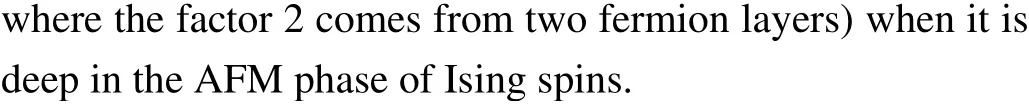
The lattice models of such quantum critical metals have a generic form. For example,in Ref.[32],the authors design a square lattice AFM model with two fermion layers and one Ising spin layer in between,which is shown in Fig.1(a). The Hamiltonian is given as


In a series of of Refs.[30–32]the authors have established the nFL self-energyω1/2n,bosonc susceptibilityχ−1(q,Ωm)∼(q2+Ωm)1−η,the anomalous dimensionη ∼1/Nh.s.roughly consistent with the HMM theory and its higher order perturbative renormalization group analyses.[10,89]However, as we will explain in the Subsections 2.3 and 2.4 below, to numerically obtain these results requires careful analysis and we have also seen signatures beyond the one-loop perturbative RG calculations. Whether the other fixed points, proposed for such type of AFM QCP withz=1[20]and their possible numerical investigations[90]can be verified, still remains an open question.
Compared with the model of the antiferromagnetic Ising quantum critical metal, the ferromagnetic quantum critical metals we studied consist of three similar terms. Here, we introduce two similar ferromagnetic models, with quantum Ising spin[33–35]and quantum rotor[37,38]coupled to fermions,respectively.The free fermion part remains two layers to avoid the sign problem,two spin flavors offering degenerate FS geometry. After certain unitary transformation without changing the values of weights, the matrix elements of the two layers are complex conjugate to each other, that is, the corresponding weights are complex conjugate to each other,and the total weight is a positive real number. There is no sign problem here. The bosonic degrees of freedom are ofZ2and O(2)symmetries,corresponding to the Ising andXYcases,with the latter replaces the original separate rotation of fermions and the Ising spins to the joint rotation of fermions and rotors and renders the OP non-conserved. The coupling termHIntis onsite,leading to criticality on the entire FS.The Hamiltonian of the Ising coupled fermions follows Eq.(2),where we setJ<0.For rotor coupled fermions, we haveH=Hf+Hrotor+HIntwith
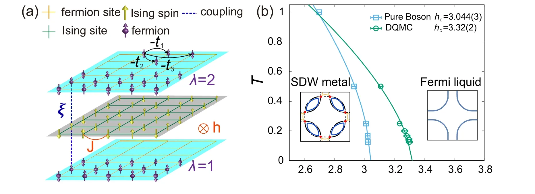
Fig.1.(a)Lattice model for antiferromagnetic quantum critical metal.Fermions reside on two layers(λ =1,2)with intralayer nearest-,second-,and third-neighbor hoppings t1,t2,and t3. The middle layer is composed of Ising spins,subject to nearest-neighbor antiferromagnetic Ising coupling J and a transverse magnetic field h. Between the layers,an on-site Ising coupling ξ is introduced between fermion and Ising spins. (b)Phase diagram of the model. The light blue line marks the phase boundaries of the pure bosonic model HIsing, with a QCP (light blue circle) at hc =3.044(3)with 3D Ising universality. After coupling with fermions,the QCP shifts to higher values. The green solid circle is the QCP obtained with DQMC(hc=3.32(2)). The system sizes in the DQMC simulations are upto 28×28×200. The figure is adapted from Ref.[32].

Without the coupling term,the bare rotor model exhibits quasi-long-range ferromagnetic order at smallU/tb. Conversely, at largeU/tb, the rotors degenerate to individual degree of freedom on each lattice site,which represents the disordered phase. The two phases are bridged via a Kosterlitz–Thouless transition. The quantum Monte Carlo simulation of the quantum rotor model has been discussed thoroughly in Ref. [36]. When tuning on the coupling strength, gapless excitations near quantum critical points drive fermions to develop effective interactions, and change rotors dynamics as well.In our studies,[37,38]we fix the FS geometry by assigningt1=1,t2=0.2,t3=0,µ=0,to avoid nesting. Besides,we settb=1, and changeUand temperatureTto obtain the phase diagram. Note that the different choice ofKleads to totally distinct physics. Here,we consider two values,K=1,4,giving rise to the nFL behavior and pseudogap,superconductivity behavior at intermediate temperature scales. We will focus on these results in Subsections 2.2 and 2.3.
2.2. Pseudogap and superconductivity near ferromagnetic critical point
First, we show the phase diagram atK=1,4 in Figs. 2 and 3. As described in Eq.(3),we set large coupling strengthK=4 to produce effective pairing for fermions. AtK=1,the superconducting fluctuations are not detected untilT=0.05.Previous studies[91–94]of spin-fermion model also observed similar superconducting dome near quantum critical point.However, in our study, we identify a pseudogap phase that was never observed in such a spin-fermion model. To carefully study the properties of these phase diagrams, primarily, we measure correlation functions of Cooper pairs in various pairing channels, including s-wave and p-wave, intralayer singlet and triplet, spin-singlet and triplet. We find that the dominant pairing channel is the on-site, s-wave, layersinglet, spin-triplet, with total spinS=0, written as∆(r)=

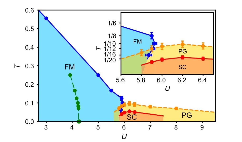
Fig. 2. The T–U phase diagram of coupling strength K =4 rotor coupled fermions model. Blue region represents ferromagnetic/superfluid phase of rotors. Blue dots with solid line(green dots with dashed line)are the phase boundary of coupled(bare)rotor model,which are determined by the superfluid data collapse. Yellow and red regions denote pseudogap and superconducting phase of fermions, respectively. The upper boundary is estimated by identifying the onset of the gap of fermionic spectrum function. While superconducting upper boundary is determined by the pairing susceptibility data collapse.Superconducting fluctuation is enhanced,since K is large,and so-called pseudogap region appears. On the other hand for bosonic part,the phase boundary bends over at low temperature,giving rise to the re-entrance phenomenon of superfluid phase. The figure is adapted from Ref.[38].

Fig. 3. The T–U phase diagram of K =1 rotor coupled fermions model.Compared with K = 4 in Fig. 2, the superconducting fluctuation is suppressed in the temperature range we studied, which is convenient for us to explore nFL behavior. The putative QCP is shown as red dots at U =4.3.Regions I and III denote ferromagnetic and disorder phases for bosonic part.The phase boundary is determined by the susceptibility data collapse at fixed temperature. nFL labeled region II appears near QCP, where the quantum part of self energy satisfies ∼ω1/2n . The figure is adapted from Ref.[37].

Subsequently,we focus on the temperature scales higher thanTc. Former studies showed nFL behavior,[32,33]which is similar to the cuprate phase diagram.The most direct way is to examine the single particle density of states. Nonetheless, in our model, due to strong bosonic fluctuation, we assume that there exists a pseudogap region surrounding the superconducting phase. To clarify this in a most direct way, the authors in Ref.[38]compute the single particle density of states in QMC simulation, imitating the angle-resolved photoemission spectroscopy (ARPES) experiments results.[95,96]They calculate the local Green’s function along imaginary axis and perform the analytic continuation[97–100]and finally obtain the results in real frequency shown in Fig.5. Remarkably,when focusing on the onset of the full-gap nearω=0, one finds the consistent temperature approximately atT=0.05,comparable with that ofTc.

Fig.4. Data collapse of pairing susceptibility following KT scaling behavior, Ps =L2−ηc f(Le−A/(T−Tc)1/2), where ηc =0.25, f is a universal function. The best fit gives A=0.075 and Tc =0.048. The figure is adapted from Ref.[38].
Fig. 5. Local density of states at U =6.0 and L=12 for various temperature. The fermionic state goes through nFL, pseudogap, and superconducting state,corresponding temperature ranges T >0.1,0.1>T >0.048,0.048>T.At nFL state,the spectrum has no minimum near ω=0,indicating high-temperature continuum behavior. The onset of pseudogap behavior is identified by existing local minimum near ω =0,corresponding T =0.1 in the spectrum. Decreasing the temperature, the gap exhibits gap-filling evolution,instead of gap closing for conventional superconductor.At lowest temperature, full gap appears, as in the superconducting phase. The figure is adapted from Ref.[38].
It must be stressed that the pseudogap region here is not directly comparable with the pseudogap phenomenon in cuprate high temperature superconductors,since we are working in a ferromagnetic QCP regime rather an antiferromagnetic one. Besides, the cooper pairs in this model possess s-wave symmetry,instead of p-wave symmetry near nematic QCP,or d-wave near antiferromagnetic QCP, which results from the isotropic FS, in contrast with the nodal-antinodal structure.Generally,the first appearance of the high-temperature gap at the antinodal momentum is identified as the onset of pseudogap behavior. In view of this,we determine the upper boundary by observation of density of states curve to find whether there exists a minimum near fermi energy.In Fig.4 atU=6.0,we findTPG∼0.1. TuningU, we obtain one crossover line shown as the yellow dashed line in the phase diagram,whose maximum is also located near QCP.
Another way to estimate the upper boundary of the pseudogap region comes from the Eliashberg equation. Within this theory, one solves the set of self-consistent equations for fermionic self-energy and bosonic propagator, with the latter as the input information and obtained by the numerical simulation. We further map the whole model with theγmodel of theoretical analysis and findTPG=0.08. Note here,theγ-model is a theoretical quantum-critical model for which the dynamical four-fermion interactionV(q,ωn)= ¯gγ/|ωn|γ,where ¯grepresents effective four-fermion interactions. Our model corresponds toγ=1/3 model,[101]where the results of the Eliashberg equation givesTPG=4.4¯g. We calculate ¯gwith respect to the simulation results of self-energies, and finally getTPG=0.08,which is in good agreement with the measurement ofTPG=0.1 atU=6.0.
BetweenTPGandTcis the region which we regard as the pseudogap phase. In contrast with the conventional superconductors,the temperature evolution of the fermion spectral gap follows a gap-filling regime, instead of a gap-closing regime.The density of state remains finite atω=0.
To further study the temperature scales of the pseudogap region, we calculate the superfluid densityρs. In such model,ρsis used for determining the approximate onset temperature of pseudogap, as it reaches the universal coefficient 2π/T,shown in Fig.6 and we obtain the temperature scale ofT ∼0.1,consistent with theTPGdiscussed above.
To sum up,we identify a pseudogap region aboveTcand determine its phase boundary primarily by observing single particle spectrum structure,assisted with other observables.

Fig.6. Superfluid density ρs versus temperature at U=6 for various system sizes.The onset temperature of superconducting fluctuation is approximated by the crossover temperature for curve of ρs(L →∞) and linear function with slope 2/π. For studied system size, we estimate such temperature is at the scale of T ∼0.1,consistent with the onset of pseudogap in the phase diagram of Fig.2. The figure is adapted from Ref.[38].
2.3. The nFL behavior and fermionic self-energy analysis
AboveTc, the fermions near QCP exhibit incoherent properties, which is regarded as the nFL state. To construct this state in a lattice model, reminiscent of prior chosen coupling strengthK, we expect it is more convenient to study the nFL in the smallKregime, where the superconducting fluctuation is greatly suppressed. We takeK=1 rotor coupled fermions model in Eq. (3), accompanied by Ising coupled fermion model in Eq.(2)as two examples,whose phase diagrams are shown in Figs.3 and 7.fermion–boson coupling,and satisfies ¯g ≪EF,which provides data forΣ(ωn)for a substantial number of Matsubara points in the rangeωn ≫Σ(ωn). For this reason,vertex corrections that contribute toΣcan be neglected in this regime. These conditions simplify the solving process of Eliashberg equations.[102]

Fig.7. The T–h phase diagram of Ising coupled fermions model, which is similar to the phase diagram in Fig.3,where both nFL state,ferromagnetic and disorder phase exist. The difference comes from the nFL state, where in this case,the quantum part of self energy satisfies ∼ω1/2n . The figure is adapted from Ref.[33].
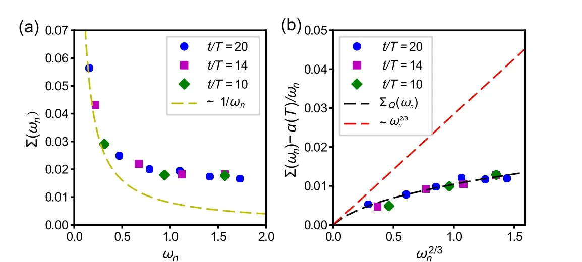
Fig. 8. Self energy analysis of Ising coupled fermions model. (a) The self energy versus Matsubara frequencies ωn at various temperatures,where clear 1/ωn behavior (shown in dashed line) is observed at small ωn. (b)Subtracting contributions of thermal part,y-axis reviews quantum part contribution.x-axis is set to be ω2/3,and red dashed line is guided to the eyes as ΣQ ∼ω2/3.Numerical data of solid dots fall on the black dashed line,which asymptotically approaches ∼ω2/3. The figure is adapted from Ref.[35].
In early studies, the ferromagnetic critical point was explored by integrating out fermions departure from FS in the effective action and obtaining the effective Lagrangian for bosonic degrees of freedom,known as HMM theory.[4–6]The theory predicts nFL states near QCP,and the change of critical exponents and university class from the pure bosonic theory.Hertz’s calculation found the dynamic critical point near ferromagnetic QCP isz=3.To verify the nFL behavior,an obvious judgement is the quasi-particle weight,which approaches zero as temperature goes down. Numerical studies in Ising fluctuation coupled with free fermions clearly show this feature.[4]Next,we focus on the fermionic self-energy.We plot the imaginary part of self-energy ImΣversus fermionic Matsubara frequencyωn=(2n+1)πTin Fig. 8. It is well known that in a FL state,the self energy is linearly proportional toωn,contributing to the quasi-particle weight. Here, we find at smallω,ImΣdiverges approaching zero frequency. To explain this,we use the Eliashberg equation to calculate the explicit expression ofΣ. In the first place,we have the following relations in such coupling strength:

where ωF/ωb is fermionic/bosonic crossover frequency scale where the self-energies change its power law behavior. ωF ≪ωb guarantees the studied Matsubara frequencies ωn is much smaller than ωb. Therefore, shown as following, one can expand Σ with the power of ωn/ωb. Besides, ¯g is the effective
Our way to deal with the divergence is to separate the contribution of quantum part and thermodynamics part, indicated asΣ(ωn)=ΣT(ωn)+ΣQ(ωn). The so-called thermal partΣT(ωn)is the contribution from static thermal fluctuations and possesses the formΣ(ωn)=α(T)/ωn. Simply speaking,the finite temperature due to the Monte Carlo simulation characters introduces a finite gap, with the gap being the coefficients, playing the role ofα(T). Therefore, at zero temperature, theΣTterm vanishes. The 1/ωnbehavior can be examined by a few smallest frequencies. ForΣQ(ωn),the quantum part contribution comes from dynamical bosonic fluctuations.At zero temperature,Σ(ωn)=ΣQ(ωn) is just the fermionic self-energy at QCP,indicating nFL behavior.
One needs to solve the following self-consistent Eliashberg equation:

Here,Nf=2 is the number of fermion flavors.Π(q,Ωm)is the bosonic self-energy solving by the free fermions propagator.D(q,Ωm)is the bosonic propagator,which can be extracted by calculation of dynamic susceptibility, along withΠ(q,Ωm),whileG(q,ωn)is the free fermionic propagator.
On the condition when the total spin alongz-axis is conserved,e.g.,Hamiltonian like Eq.(2),we find the leading order ofΠ(q,Ωm)∼|Ωm|/q, known as the Landau damping term calculated using Eq. (5). Bringing the fermionic selfenergy calculation, eventually we obtain the analytic formula ofΣ(kF)atωn ≪ωbregime as

which indicates the fermionic self energy is∼ω2/3nand deviates from the Fermi liquid behavior.

whereχ0,M0,Γ0are all extracted from the Monte Carlo simulation results. Note in the next subsection, we will give a detailed description of such formula. Equation (7) considers high-order diagramatic representations, which is different from the first-order calculation in Eq.(5). Especially, the coefficientsχ0,M0,Γ0are obtained by fitting the bosonic dynamical susceptibility data in Monte Carlo simulations. Repeating similar calculation for solving fermionic self-energy as Eq. (5), we finally get fermionic self-energyΣQ(ωn)∼ω1/2nin Fig.9,which is also a nFL behavior. It needs to be noticed that,only in small coupling strengthKfor rotors and fermions,e.g.,K=1,one can separate the thermal and quantum parts ofΣ(ω).[37]
In antiferromagnetic model,it was hard to directly reveal the scaling form of the nFL self-energies.
Ath Fig.9. Self-energy analysis of rotor coupled fermions model in Eq.(3). (a)The self energy versus Matsubara frequencies ωn at various temperatures,where clear 1/ωn behavior(shown in dashed line)is observed at small ωn.(b) Subtracting contributions of thermal part, y-axis reviews quantum part contribution. In contrast with the Ising coupled fermions model, x-axis is set to be ω1/2,and the dashed line is guided to the eyes as ΣQ ∼ω1/2. Numerical data of solid dots fall on the black dashed line,which asymptotically approaches ∼ω1/2. The figure is adapted from Ref.[37]. Fig. 10. Fermionic self-energy for antiferromagnetic fluctuations coupled fermions. (a)On the Fermi pockets,the system is in a Fermi liquid state as shown by the linearly vanishing of Im(Σ(k,ωn)) at small ωn. At the hot spot, due to the Fermi surface reconstruction, an energy gap opens up, resulting in a divergent Im(Σ(k,ωn)). (b) On the Fermi pockets, the system remains a Fermi liquid as shown by the linearly vanishing Im(Σ(k,ωn))at small ωn. At the hot spot, Im(Σ(k,ωn)) has a small but finite value as ωn goes to 0, which is the signature of a non-Fermi-liquid, but still different from the HMM expectation discussed in Subsection 2.3 and therefore remains to be explained. The figure is adapted from Ref.[32]. The bosonic propagators or bosonic dynamic susceptibilityχ(q,Ωm)also reveal important information about the quantum critical metals. Their definitions for the Ising and rotors are Generally, in such spin-fermion model, we couple free fermions to the bosons, which have their own dynamics. For the bare Ising or rotors,they both satisfy the dynamic critical exponentz=1,i.e.,the susceptibility reads whereris the tuning parameter,Mrrepresents the distance towards the QCP.Q=(0,0)for ferromagnetic and(π,π)for antiferromagnetic models,is the ordered wave vector.When tuning on the coupling between boson and fermion, the bosonic dynamics change their behavior.Previously,HMM theory predicts that the dynamic critical exponents at ferromagnetic and antiferromagnetic QCP change toz=3 andz=2,respectively.Several recent simulation results found the difference with the universality of Hertz–Millis-type exponents, indicating nonuniversal behavior near QCP.[30,32,33]Likewise,we give a detailed analysis of the results in our models. The bosonic dynamics of other cases also deserve an explanation, e.g., near QCP but covered by the superconducting fluctuations. Moreover, far from the QCP, the bosonic dynamics can be easily achieved by diagramatic calculations,such as RPA.In the subsection, we focus on the dynamic susceptibilityχnear nFL state,and plenty of situation is summarized in Table 1. Besides bare nFL state,in Subsection 2.2,we discuss the case forK=4 rotor model and find the bosonic susceptibility is influenced by superconducting fluctuation and the distance from the QCP.Below,we briefly discuss that even in this case,where the QCP is masked by the superconducting dome, the bosonic susceptibility can still reveal the different scaling behavior. Figure 11 showsχ−1(q=0,ω)−χ−1(q=0,ω=0)for differentU. We chooseU=3.0 (ferromagnetic phase),U=6.0 (near QCP),U=8.0 (disordered phase), to demonstrate the joint effect of superconducting fluctuation,fermionic self-energy and non-Landau damping behavior. ConsideringUis far fromUc, first we draw attention toU= 8.0. At bosonic Matsubara frequenciesΩn>1,χfollows RPA calculation with respect to free fermions propagators. The behavior is reminiscent of Ising coupled fermions model,as the similar non-analytic function∆(q,ω)in Table 1 1a. At small frequencies,χdeviates from the nonzero extrapolation,since the fermions enter the pseudogap region at low temperature.Similar thing manifestes atU=3.0, where on log–log scale,the slope of 2(correspondingz=1)behavior is the proper description of ferromagnetic phase.Due to the spin gap,the coupled model evolves like bare rotor model,and has no intercept in ferromagnetic phase. However, atU=6.0 near QCP, we separate theΩregion into three parts according to the temperature region. At largeΩ, corresponding toT>0.1, the bosonic self-energies follow non-Landau damping regime and satisfyz=2 (slope is of 1), similar to the expression of Table 1 1b. Towards low frequencies, the dominant pseudogap region drivesz=2 toz=1. At lowest temperature studied,because of the superconducting gap,the behavior goes back to the bare rotor model withz=1. There are still many open questions in the study of quantum critical metal. The results summarized in Table 1 for dynamical critical exponentz, are largely consistent with the HMM prediction, for example, when the bosonic order parameters are conserved(Ising spin),one obtainsz=3 for the ferromagnetic QCP,z=2 for antiferromagnetic QCP bosonic self-energies,and only when the bosonic order parameters are not conserved (rotors with O(2) symmetry), one would need higher order perturbative calculation beyond the HMM theory to obtain thez=2 bosonic self-energy.[22,37,38]However,there are many predictions that the antiferromagnetic bosonic fluctuations coupled fermions will eventually deviate from the HMM form and new fixed points could be found,wherezhas strong violations fromz=2.[20,89]At the present stage of the model design and computation, such deviations are yet to be unambiguously found. For example,we find in Ref.[32]that the predicted rotation of the renormalization fermion velocity towards the IsingQAFwas not as obvious as the theoretical prediction to be parallel. Table 1. Summary of quantum critical bosonic self-energies for the systems in the review. q is the momentum measured with respect of the ordered wave vector Q=Γ for ferromagnetic and nematic QCPs and Q=QAF for antiferromagnetic QCP.Ω is the bosonic Matsubara frequency. Fig.11. Bosonic dynamical susceptibilities χ−1(q=0,Ωm)−χ−1(q=0,Ω0)at U =3,6,8, corresponding subfigures(a), (b), (c), respectively. The subfigures (a) and (b) are plotted on log–log scale. (a) At ferromagnetic phase U =3.0, the lowest frequencies follow the red line guided to the eye,whose slope is 2, indicating z=1 behaviors. (b) Near QCP at U =6.0, the fermionic parts go through nFL, pseudogap, superconducting state from higher to lower temperatures. On account of this, the bosonic dynamical susceptibilities exhibit non-landau damping behavior, transition period, and bare rotor model from higher to lower frequencies,corresponding the crossover from z=2(slope of 1)to z=1(slope of 2),described by the red and blue lines. (c)At disorder phase U =8.0,the behavior is similar to that in ferromagnetic phase with both z=2. The red line is the best fit of the data at Ωm>0.5,which possess square behaviors. While,a finite intercept exhibits at extrapolation of Ω =0,as the RPA calculation,where one uses free fermionic propagators.[10] At small frequencies,guided by blue lines,the bosonic part is effected by the pseudogap behavior,and deviates from the red line. The figure is adapted from Ref.[38]. Recently there are hybrid Monte Carlo simulation results[90]showing at antiferromagnetic O(3) QCP, there exist clear deviations of the dynamic exponent fromz= 2 toz ≈1.65 at the smallest nesting angle. Furthermore, a breaking of the O(2)symmetry form of the momentum dependence down toC4happens near QCP,which also violates the HMM theory. Remarkably, one recent long review[106]discussed nFL implemented on the 2d AFM QCP in field-theoretic functional renormalization group formalism. The author developed the low-energy effective field theory of nFL including all gapless modes around the Fermi surface. Through functional renormalization group flow,nFL is ascribed to the fixed point,thus its low-energy physics can be studied. These results and statements are certainly at our interests and the interests of the community for the future research activities of the sport and pastime of model design and computation in quantum critical metals. As discussed in Sections 1 and 2, the nFL behavior of interacting electron systems,is widely believed to be relevant to the microscopic origin of the “strange metal” behavior in unconventional superconductors[107–114]and many other condensed matter systems. And the nFL often occurs via electron interactions mediated by gapless bosonic modes that render the electrons incoherent.[16,30,32–34,89,115–120]In Section 2,we study many 2D lattice models where we couple itinerant fermions with soft boson mode with critical fluctuations, and then study the nFL behaviors in the vicinity of the ferromagnetic and antiferromagnetic QCPs. Due to the lack of a natural small control parameter, the analytical solution to these models remains challenging. And in order to see nFL behavior numerically,such models always require us to turn the mass of the boson to the critical value,as seen in the examples in Section 2. But the system will go back to FL behaviors once away from the QCP. The position of QCP and region of nFL are model dependent and affected by the finite-size effect. In addition, we also need to deduct the non-negligible thermal contributions to the fermionic selfenergy and control the strength of effective coupling,[35,37,121]so as to see a clear signal of nFL from fermionic self-energy.These difficulties make it hard to see the scaling form of nFL,which inspired us to design other models. Recently, nFL behaviors in Sachdev–Ye–Kitaev (SYK)models[39,122–124]have garnered widespread attention. The SYK model is an exactly solvable model initially proposed by Subir Sachdev and Jinwu Ye,and then modified by Alexei Kitaev. The motivation of the SYK model is to come up with a model to explain the phenomena of strange metal and a simple model for quantum holography.The advantage of the SYK model is that it is exactly solvable, and its exact solution is a nFL.[125]Inspired by such exactly solvable SYK models with nFL behavior, recently a class of SYK-like models featuring random Yukawa interactions between fermions and bosons has been put forward to analyze the nFL problem.[41,126–129] In this section, we will discuss our model design and computation for Yukawa-SYK model and the nFL,self-tuned quantum criticality and superconductivity therein.[42,43]It is interesting to see that the Yukawa-SYK model acquires a very unique self-tuned quantum criticality and in that the system is always inside an nFL independent of the tuning of the parameters,and the quantum fluctuations in the system also naturally give rise to the superconductivity,as we shall explain below. Compared with the SYK model that only involves interacting fermions, our Yukawa-SYK model, which is also analytically solvable in the large-Nlimit,has a dynamical bosonic degree of freedom. As shown in Fig. 12, there areMquantum dots and each hostingNflavors of fermions. Fermions of different dots interact withN2bosons via all-to-all random Yukawa interactions. The Hamiltonian[42,43]is Fig. 12. The M quantum dots labeled by {i,j} have N flavors labeled by {α,β γ,δ,...} each. Fermions in different dots are coupled to bosons through a random Yukawa coupling tiα,jβ,where bosons are given by antisymmetric fields φαβ. The figure is adapted from Ref.[42]. We find that the high-rank randomness of the Yukawa couplingtiα,jβin our model is important for stabilizing the nFL behavior. Also the spinful fermions, with the Pauli matrixσzin Yukawa coupling term,actually help us to avoid the sign problem in the QMC simulation. Sincetiα,jβis symmetric matrix andφαβis antisymmetric, the Hamiltonian is invariant under the anti-unitary transformationJ= iσyK,whereKis the complex-conjugate operator. Or to put it simply,the matrix elements of different spins are all Hermitian to each other,so no sign problem in the evaluation of the fermion determinants.[42,83] The major difference between the Yukawa-SYK model and those in Section 2 is the random all-to-all coupling.Within the large-Napproximation, the Yukawa-SYK model is “selftuned”to quantum criticality.The system becomes critical,independent of the bosonic bare massm0. This means we do not need to adjust the parameters close to QCP to study nFLs. Despite this benefit,there are also costs:all-to-all coupling makes the computational complexity of QMC increase fromO(βN3)toO(βN5M3). Since it is not on-site boson–fermion coupling,the Sherman–Morrison formula for efficiently computing the matrix inversion[130–133]does not apply in this case, which makes the computational complexity of weight calculation and updating Green’s function change fromO(N2) toO(N3M3).This is because the Yuakwa-SYK model hasN(N −1)/2 independent bosonic fields at each time slice, instead ofN, while the number of time slices is proportional toβ. In addition,because random termstiα,jβexist, we need to perform multiple Monte Carlo processes to achieve the disorder-average,on top of the regular Markov chain for each set of{tiα,jβ}. Through numerical simulation of QMC and large-Ncalculation, we obtained the global phase diagram of Yukawa-SYK model, as shown in the Fig. 13. By solving the linear Eliashberg equation using the large-Nresult of the Green’s functions and considering the pairing susceptibility data in QMC simulations, a finite temperature phase transition from nFL to superconductivity can be seen in some intervals of the chemical potentialµ. And we can see that by solving the Schwinger–Dyson equation, the first-order quantum phase transition extends to low temperature and terminates at a (thermal) critical point, which is common in lots of metal–insulator transitions in correlated materials.[134,135]And the reason for choosing two different sets of parameters is that the superconducting dome completely preempts the wouldbe nFL/insulator transition forN= 4M,ω0= 1,m0= 2(Fig. 13(a)), while forN=M,ω0= 1,m0= 2, the firstorder phase transition is stronger and the corresponding thermal critical point occurs outside of the superconducting phase(Fig.13(b)). Fig. 13. (a) Global phase diagram of the spin-1/2 Yukawa-SYK model at N=4M,ω0=1,m0=2.From the large-N calculation,over a wide range of chemical potentials µ, we can see a finite-temperature transition from nFL to SC, until the chemical potential increases to the line where a first order superconductor-to-insulator phase transition occurs. The first-order hysteresis region is denoted by the red points and lines. The thermal critical point that terminates the first order transition locates at(µc=0.194,Tc=0.015).And the blue triangles are the transition points from nFL to superconductor obtained from QMC at finite N =4M, which are consistent with the large-N calculations(black squares). (b)Global phase diagram of the spin-1/2 Yukawa-SYK model at N =M,ω0 =1,m0 =2 from the large-N calculation. Similarly, large-N calculations will give the first-order hysteresis region, while the dashed-line portion of this boundary means it is renormalized by superconductivity phase. The QMC n–µ parameter scans in Fig. 14 are along the blue dashed paths. The thermal critical point at(µc=0.3825,Tc=0.07)is denoted by the black star. The figure is adapted from Ref.[43]. One can slove the Yukawa-SYK model at theN,M →∞limit analytically,[41,126–128]by following the original treatment of the SYK model.[39,122–124]In this limit we have the Schwinger–Dyson(SD)equations After iterative solution of Eq.(11)(introducing the“stabilizers”for each step of the iteration[43]),we obtain the hysteresis region which separates nFL from insulator(red lines in Fig. 13). And we can get fillingnsince we have imaginarytime fermionic Green’s function from QMC and the solution of Eq.(11): Figure 14 shows the exact (n,µ) curve in different parameters. The coexistence of two solutions for certain(µ,T)indicates a metastable state. Similar to the water–vapor transition,then–µcurve connecting the two branches is a straight line determined by the Maxwell construction. The two types of solutions become smoothly connected at a chemical potentialµcabove a certain temperatureTc. Here(Tc,µc)is a thermal critical point of the system, for that the compressibility dn/dµdiverges. The parameter transformation range in Fig. 14 corresponds to the blue dashed line in the phase diagram,Fig.13(b).The fillingnis doubly valued in the hysteresis zone(a range ofµ)at lowerT. The nFL behavior is represented by the lower branch,while the insulating behavior is represented by the upper branch;a first-order transition connects the two at a chemical potentialµc=0.3825,which is denoted by the black star.The dashed line marks the boundary between stable and unstable solutions. Fig.14. Filling n versus µ for certain T in the vicinity of the thermal critical point in Fig.13(b)for N=M,ω0 =1,m0 =2. Both QMC and large-N results are shown in the figure. At higher temperature T,one sees the n(µ)curves both from large-N and QMC are smooth,while T =0.125,µ=0.375(marked by the star),is a thermal critical point. At temperature T =0.083,which is close to the thermal critical point, a sharp turn of n(µ) signifying the divergence of the compressibility dn/dµ can be seen. At lower T,there is a range ofµ —the hysteresis region—where the filling is doublevalued. The upper branch represents the insulating behavior and the lower branch represents the nFL behavior. A first order transition connects the two branches at a chemical potential given by a Maxwell construction. The dashed line delimits the region where solutions are unstable. The figure is adapted from Ref.[43]. In Refs.[126,127],some large-Nresults have been found that whenT= 0,µ= 0, form0∼ω0andω,Ω ≪ω0, the fermionic and bosonic self-energies are given by Here it is worth noting that the Fourier transform forΠ(Ω)shall be carried out carefully, this is because the positive power-law|Ω|1−2xdoes not have a Fourier transform in the common sense as the Fourier integral is UV divergent for 0 In our Yukawa-SYK model, at a finite but low temperatureT=1/β ≪ωF=ω30/m20,the long-time correlated behavior persists.[39,122–124,126,127]By applying a reparametrization symmetry transformation[39,122–124]τ →f(τ) = tan(πτ/β),we know that at low temperatures and long-time limit, It was already well known that in the SYK model, the fermion Green’s function is incoherent:[39]G(τ)∼τ−1/2at largeτ, while in FL the quasiparticles have the coherent Green’s function:G(τ)∼1/τ. And whenT>0, the SYK Green’s function has conformal invariance as follows:G ∼(T/sin(πkBTτ/¯h))1/2.[136] Back to our spin-1/2 Yukawa-SYK model,the exponentxis between 0(same as in a noninteracting disordered electron system)and 1/2(same as in the SYK model). The power-law behavior of bosonic and fermionic Green’s functions both in the Matsubara frequency and imaginary time, can be used to identify the nFL behavior. The question for the QMC simulation of the Yukawa-SYK model is to explore whether at small and finiteMandN, where the perturbative analysis no longer works, the system could still exhibit the nFL behavior as in Eqs. (13) and(17), and whether there will be emergent symmetry breaking phases such as superconductivity generated by the quantum fluctuations in the nFL. These questions, as we shall see below, have been answered affirmatively by our model design and computation. According to Eq.(17),we can look for the nFL fermionic and bosonic Green’s functions directly in the imaginary time decay. In Fig.15,we present the log–log plot of the behavior ofGfandGbatN=4M,ω0=1,m0=2,µ=0, and different temperatures from iterative theoretical calculation. Here for 4M=N, one findsx ≈0.231. The solution of Eq. (17)matches well in the long-time limit with the approximate result obtained using time-reparametrization symmetry,exhibiting self-tuned criticality and nFL behaviors. The system behaves as a quantum critical NFL, with a pairing instability atTc<ωF. Fig. 15. Theoretical result of Gf and Gb at N =4M →∞, ω0 =1,m0 =2,µ =0. When β is very large,the solution of the SD equation agrees very well with the analytic form in Eq.(17).The figure is adapted from Ref.[42]. Fig. 16. QMC results at N =4M, m0 =2,ω0 =1,µ =0 and β =16 for M=2,3,4. (a) and (b) Green’s function Gf(τ,0) and Gb(τ,0) versus τ in the range of τ ∈[0,β]. Blue, red and yellow dots are DQMC data and the black dashed line is the large-N result. (c)and(d)The same as above, but in a special log–log scale The convergence towards the large-N results as(M,N)increase is obvious. The figure is adapted from Ref.[42]. Fig.17. The QMC fermionic Green’s functions(a)and the bosonic Green’s functions(b)with differentµ. M=4,N=16,β =32,ω0=1,m0=2. For convenience both the Gf and Gb have been normalized to 1 at τ =β. The system becomes gapped with the increase of the chemical potential. Note that the sharp downturn of the large-N result in panel (a) is an artifact of keeping finite frequency points. The figure is adapted from Ref.[43]. In addition,when we considerµ/=0 case,the agreement is also excellent.It is shown in Fig.17.Since there is no longer particle–hole symmetry, fermionic Green’s functionGfis not symmetric with respect toτ=β/2,and we normalize the data with respect toGf(τ=β)here. Whenµ=0.125,power-law decay in imaginary time ofGfandGbis seen, which is similar to that in Ref. [42]. At larger dopingµ=0.35, bothGfandGbdecay exponentially,consistent with insulating behavior discussed before. And considering finiteN,M,the system does not develop superconductivity atµ=0.35,since it is in the gapped insulator phase. So it is sensible to compare it with Green’s functions at largeNfor the normal state. Self-tuned quantum criticality means the system becomes critical due to the strong mutual feedback between the bosonic and fermionic sectors, independent of the bosonic bare massm0. From Eq.(13)we have which means the boson is critical/gapless no matter what the bosonic bare massm0is, the system renormalizes it to zero via interaction effects. This has been proved to be true in Refs.[126,127]at the large-Nlimit. Figure 18(a) shows the bare bosonic Green’s function generated from the bosonic part in Eq. (10), with the massm0=1 andβ=16.Then the Green’s function clearly exhibits exponential decay in imaginary time toGb(τ=β/2,0)≈0.However,as shown in Figs.18(b)and 18(c),once coupled with fermions in our model,the bosonic Green’s functions become critical. These results reveal the self-tuned quantum criticality in our system. The QMC data in Fig.18(c)are very close to the theoretical result. The self-tuned quantum criticality is consistent with analytical predictions at largeN.Fig.18.Self-tuned quantum criticality with different boson masses.Blue dots are DQMC data and the red dashed lines are large-Nresult(following Eq. (17)). It is clear to see power law decay ofGbat low-temperatures and long-time limit in log–log plot. These results reveal the self-tuned quantum criticality in our system. The figure is adapted from Ref.[42]. We can see that in the phase diagram shown in Fig.13(a),N=4M,ω0=1,m0=2,in low temperatures the systems are in superconducting phases in a range of chemical potentialµ.And whenµincreases, theTscis moderately reduced until a sudden drop at largerµ. The QMC results and large-Ncalculation give us the criticalµc=0.25 at zero temperature,which coincides with each other. Details will be shown below. Forµ= 0, the pairing problem was analyzed in Ref. [42], since there is particle–hole symmetry. Fermionic Green’s functionGf(τ) is symmetric with respect toβ/2. Now the Eliashberg equation is given by Φ(ωn) =ω30T∑Ωm Gb(iΩm)|Gf[i(ωn+Ωm)]|2Φ(ωn+Ωm). If we view the Eliashberg equation(19)as a matrix equation/an eigenvalue problem,we can solve for the critical temperaturesTc. As the temperature lowers, the eigenvalues of the kernel increase, andTccorresponds to the temperature at which the largest eigenvalue approaches 1. Fig.19. Pair susceptibility Ps measured at different chemical potential µ. The obtained Tc (βc)are denoted by the blue triangles in Fig.13(a). From the temperature dependence of the Ps with different system sizes(M,N)the authors in Ref.[43]perform the data collapse using mean-field exponents γ0 =1, ν0 =2 and the transition temperatures Tc (βc) are obtained accordingly. The parameters are N =4M, ω0 =1, m0 =2. µ =0 in (a) and (b);µ =0.05 in(c)and(d); µ =0.125 in(e)and(f); µ =0.2 in(g)and(h); µ =0.25 in(i); µ =0.35 in(j). The superconducting transition temperature reduces as µ increases. For µ =0.25 (i) and µ =0.35 (j), the pairing susceptibilities are not divergent at larger N, and the system enters a gapped insulator phase. The figure is adapted from Ref.[43]. On the other hand, we have the following understanding:if the system breaks the replica symmetry,the true ground state is then a spin glass. For example,in some bosonic SYK models,[141,142]there is replica symmetry breaking, and in fact it has been shown recently that similar situations occur for all random interacting bosonic models.[143–145]While for the fermionic SYK model, it seems that a glass phase is absent and the nFL state persists down toT=0.[141,142]Since our Yukawa-SYK model involves both fermions and bosons,whether there is spin glass is a question. To properly address this question, we can construct a model in a similar form of Eq.(10)but the random coupling is now of a lower rank, In Fig. 20, we show the static component (withΩm=0) for bosonic Green’s functionGb(Ωm), obtained from the QMC simulation of Eq.(22). The component can be regarded as an Edwards–Anderson order parameter of the spin-glass phase[142]in the large-Nlimit. AsNincreases,the static component, along with its variance for different disorder realizations,increases with the increase inNatM=N,β=16,andm0=ω0=1,which is indicative of spin-glass behavior. Fig.20. We show the static component (with ωn =0)for bosonic Green’s function Gb(ωn). This component can be viewed as an Edwards–Anderson order parameter of the spin glass phase in the large-N limit. As N increases,the static component, as well as its variance for different disorder realizations, increases with the increase of N at M = N,β = 16,m0 = ω0 = 1,indicating a spin glass behavior. The figure is adapted from Ref.[42]. In contrast, we can see that in Fig. 21, similar data of Eq.(10)show that our Yukawa-SYK model is not spin glass,since results ofGfandGbshow self-average of different realizations and the difference between the QMC obtained Green’s functions and the large-Nsolutions decreases with the increase ofM,N. Besides the Yukawa-SYK QMC studies presented in Subsections 3.3, 3.4 and 3.5, there is also new QMC research on complex SYK model,[146]where it was found one can design the similar model like our Yukawa-SYK with only fermions without the sign problem, and it is shown that the self-tuned and nFL behaviors also persist. Fig.21. QMC bosonic and fermionic Green’s functions Gb and Gf, which are from 20 different disorder realizations with M=N=9,β =24,m0=2 and ω0=1,are shown in(a)and(c). And(b)and(d)present the difference between theoretical (large-N) results GTheory(β/2,0) and QMC numerical simulation data G(β/2,0). The figure is adapted from Ref.[42]. Quantum Moir´e systems such as TBG and TMD systems,bestowed with the quantum geometry of wavefunctions–manifested in the distribution of Berry curvature in the flat bands–and strong long-range Coulomb electron interactions, exhibit rich phase diagram of correlated insulating and superconducting phases thanks to the high tunability by twisting angles,gating and tailored design of the dielectric environment. The extremely active research field of 2D quantum Moir´e materials is developing very fast.[44–77] The theoretical efforts, from model design to the computation solutions in the quantum Moir´e lattice models are also moving forward rapidly. The real space effective lattice models give rise to the proper description of the ground state insulating phases with various symmetry breakings patterns and the topological nature has been obtained both from the mean-field type analysis and quantum Monte Carlo and tensor-network many-body computations.[57,58,68,85–87,154–157] Later on,it was understood that due to the quantum metric in the flat-band wavefunction and the 2D long-range Coulomb interactions,the proper description of the quantum Moir´e lattice model shall be constructed in continuum in momentum space. And it is from here the exact solutions at the chiral limit[158,159]and mean-field analyses of the ground state phase digram[157,160–162]and the momentum-space quantum Monte Carlo algrithm[78,79,163]to solve these systems and their intricate Monte Carlo sign structure[82–84]have been gradually and successfully revealed. Many interesting properties of the quantum Moir´e lattice model have been discovered ever since and people gradually find many evidences[86,87]pointing to the fundamental difference between the correlated flat-band lattice model and those of the conventional correlated electron lattice models systems,such as Hubbard-type models, in that, the interplay of topological wavefunction and long-range Coulomb interaction not only gives rise to complex ground state phase diagrams with possibly different pairing mechanism and symmetry breaking patterns,[80]but also hints at the difference in their thermodynamic and dynamic responses.[81] Since the field of quantum Moir´e materials is developing very fast, it is nevertheless not the purpose of this section to present an exhaustive survey of all the efforts in the understanding of the rich physics of quantum Moir´e materials, but mainly focus on the model design and computation solutions inspired by the fast development of the field,and in a mutually constructive manner, demonstrate how our attitude of a sport and a pastime of doing so, actually either solve the present mysteries or point out the new directions that await to be explored. To properly take the long-range Coulomb interactions into consideration in the Moir´e system and explain various correlated insulating phases at the integer fillings such as the quantum anomalous Hall and intervalley-coherent insulators,one would need to start with the continuum model at momentum space, i.e., the Bistritzer–MacDonald (BM)[44–46]type of model and project the Coulomb interactions onto the flatbands while at the same time including the renormalization effects of the remote bands. The difficulty of doing so lies in the fact that there are no generic quantum many-body approaches that handle the long-range interactions well, except Hartree–Fock-type mean-field calculation[157,161,162]and ED for very small cluster,[164]and this is the reason that inspired us to successfully develope the momentum-space quantum Monte Carlo method for this purpose,[78,79]which we will particularly focus on in later sections. But before going directly to the continuum model, one can still construct a real-space lattice effective model at the Moir´e scale which captures the extended interactions beyond the Hubbard-type local interaction,[154–156,165,166]and develop controlled quantum many-body numerical methods such as QMC,DMRG and tensor-network approaches to solve them and determine the phase diagram. This is indeed the successful path taken by many (including us) and different topological phases and intervalley-coherent phases have been identified.[57,58,68,85–87] As shown in Fig.22,we design a QMC method that can simulate the real-space lattice model with extended charge and assisted hopping interactions,with the Hamiltonian Fig. 22. (Left) The effective model with two valleys (red and green triangles) and spins and spin-valley SU(4) symmetry. The interactions act on every hexagon and consist of the cluster charge term Q and the assistedhopping interaction term T. (Right) Ground-state phase diagram, spanned by the U/W and α axes, obtained from QMC simulations. The y-axis at U =0(dashed line)stands for the Dirac semimetal phase. At small U,the ground state is a quantum valley Hall(QVH)phase characterized by emergent imaginary next-nearest-neighbor hopping with complex conjugation at the valley index,as illustrated by the red and green dashed hoppings with opposite directions. Upon further increasing U,an inter-valley-coherent(IVC)insulating state is found, which breaks the SU(4) symmetry at every lattice site by removing the valley symmetry. Since it preserves the lattice translational symmetry,it is ferromagnetic-like. The cVBS insulator,which appears after the IVC phase, breaks the lattice translational symmetry and preserves the on-site SU(4) symmetry. The IVC phase is stable at strong coupling limit. This figure is adapted from Ref.[68]. The QMC simulation results are summarized in Fig. 22(right). We find that even very small interaction values trigger a transition from the non-interacting Dirac semi-metal phase to an insulating state. Upon increasingU, the nature of the insulator changes from a non-symmetry-breaking topological QVH phase, to an onsite SU(4)symmetry-breaking intervalley-coherence(IVC)insulator,to a translational symmetrybreaking columnar valence bond solid(cVBS)phase,and then finally back to a reentrant IVC state. This rich phase diagram is a consequence of the interplay between two different types of interaction terms: a cluster-charge repulsionQand a non-local assisted-hopping interactionT. The former is analogous to the standard Hubbard repulsion and, as such,is expected to promote either SU(4) antiferromagnetic order or valence-bond order in the strong-coupling regime. The latter,on the other hand,arises from the topological properties of the flat bands in TBG.When combined withQ,it gives rise not only to SU(4)ferromagnetic-like order, but also to correlated insulating phases with topological properties,such as the QVH phase. While the precise value ofU/Win TBG is not known,a widely used estimate is that this ratio is of order 1.[156]Referring to our phase diagram in Fig. 22 (right), this means that certainly the QVH phase and possibly the IVC phase can be realized at charge neutrality,provided thatαis not too small.Experimental probes do report a gap at charge neutrality in Refs. [51,56] and the main manifestation of the QVH phase would be the appearance of gapless edge states, whereas in the case of the IVC state,it would be the emergence of aq=0 order with onsite coupling between the two different valleys. Furthermore, we also initiated the DMRG simulation at the filling factor of 3/4 of the same real-space model with extended interactions and found the quantum anomalous Hall(QAH) insulator[86,87]which is consistent with experimental findings at the same filling.These results are shown in Figs.23 and 24. The interaction-only Hamiltonian is now A quantum anomalous Hall (QAH) topological Mott insulator (TMI) with spontaneous time-reversal symmetry breaking and nonzero Chern number and a charge-densitywave (CDW) insulator have been discovered in the DMRG computation of Eq. (24).[86]We further employ the stateof-the-art thermal tensor network and the perturbative fieldtheoretical approaches to obtain the finite-Tphase diagram and the dynamical properties of the TBG model.[87]As shown in Fig.23(a),the phase diagram includes the quantum anomalous Hall and charge density wave phases at lowT, and an Ising transition separating them from the high-Tsymmetric phases. Due to the proliferation of excitons – particle–hole bound states – the transitions take place at a significantly reduced temperature than the mean-field estimation. The exciton phase is accompanied with distinctive experimental signatures such as enhanced charge compressibilities and optical conductivities close to the transition. These results explain the smearing of the many-electron state topology by proliferating excitons and open the avenue for controlled manybody investigations on finite-temperature states in the TBG and other quantum Moir´e systems. Fig. 23. (a) Finite-temperature phase diagram of the KV model, with the red regime being the high-T disorder phase,the intermediate-T orange one where exciton proliferates,the green one being the CDW phase,and the purple one being the QAH phase. The vertical dash line denotes the α =0.2 case analysed in (b) panel. (b) For the case of α =0.2, the specific heat cV data is shown versus T,where the peak at Tc =0.041 signifies the thermal phase transition. The right axis of panel(b)shows the compressibility∂n/∂µ vs. T. This figure is adapted from Ref.[87]. Fig. 24. Panel (a) illustrates the formation of exciton between two quasiparticles from the valence and conduction bands. (b) At intermediate temperature T =0.244 inside the exciton proliferation regime, the charge correlations between a central site(the asterisk)and other sites are shown here.(c) Quasi-particle spectral function Ak(ω) as the sum of valence and conduction band spectrum,for α=0.2 at T =0.08.Compared to the mean-field single-particle dispersion,which consists of upper conduction and lower valence bands (white dots), the spectral weight distribution gets broadened.The exciton band(denoted by green diamonds)lies within the single-particle gap. The corresponding path in the Brillouin zone is drawn in the inset diagram. Panels(d)and(e)show the valence electron spectral weights A vk(ω)at k=Γ and k=K for various temperatures. Panel (f) shows the gap at k=Γ and k=K as a function of temperature T. This figure is adapted from Ref.[87]. It has been found that the CDW and QAH phases are separated by a first-order transition extending from the transition pointα ≃0.12.[86]Then we turn to consider the finitetemperature Ising transition,such as atα=0.2. In Fig.23(b),the specific heatcVhas a peak atTc≃0.041, which is the evidence of a second-order phase transition from QAH to excition proliferation region at this temperature. As for the compressibility∂n/∂µ,its curve has a peak at higher temperatures aboveTc. Inside the exciton regime it also keeps an enhanced value. The above facts show the exciton(bosonic bound state)proliferation aboveTc.WhenTincreases,a crossover between the intermediate-Tand high-Tregimes will be seen. Then thecVcurve scales as the high-Tlimit ofT−2. Figures 24(a)and 24(b)show the schematic plot of the exciton excitations and its real-space presence from the densitydensity correlation functions for YC4×12 DMRG cylinder atT=0.244(aboveTc)andα=0.2 inside the exciton proliferation phase. As shown in Fig.24(b),if we place a hole at the center of the lattice, bunching and antibunching modulation behaviors of electrons are present. It is the evidence of existence of particle–hole bound states–excitons–in the system. WhenT=0.08, a representative temperature, the renormalized spectral function quasi-particleAk(ω) =Ack(ω)+Avk(ω) gives us the information of the correlated band in Fig. 24(c). Herec,vare for electrons in conduction and valence bands. Then we know that the exciton(green diamonds line) has a much lower energyEex∼0.08 than the meanfield band gap (white dots line), as shown in Fig. 24(c). In Fig.24(d)and 24(e),the spectral functions of electrons in the valence bandAvk(ω)atk=Γandk=K of different temperatures are shown. From the above data,we can see how the energy gap varies with temperature,as shown in Fig.24(f). It is clear that aboveTc∼0.04 but still below the mean-field QAH band gap atT ∼0.1, the spectral function is already gapless due to the exciton collective excitations. In order to consider the long-range Coulomb interaction and the Wannier obstruction problem,recently there have been a lot of studies to simulate TBG and other Moir´e lattice models in momentum space.[78,81,163,167]In our previous work, we start from the continuous BM model[47,168–173]and long-range single-gate Coulomb interaction,and integrate out the states on the remote bands to obtain the projected Hamiltonian[166,174] whereεm,τ(k) is the bare dispersion,[177]which is the eigenvalue ofHBM. We note that in Refs. [160,163,178,179], the mean-field contribution of the remote band interaction from the flat band is removed,which is different from our choice. We developed the momentum space QMC approaches to solve the Hamiltonian in Eq. (28), the method is free of the sign problem at charge-neutrality point (CNP) with theC2PandC2Tsymmetries,and we further proved that the flat-band system acquires a unique sign bound theory,[82]some of them,like chiral limit single valley and single spin TBG at CNP,acquires a polynomial sign problem rather than exponential,this effective means that even with the polynomial sign, the computational complexity of the lattice models such as Eq. (28)is polynomial instead of exponential and we can solve them without hitting the “exponential well”.[78,82,83]Some of the other filling cases,likeν=−1,can also be simulated in polynomial time based on the sign bound theory. With the method developed,we can now compute the detailed static, dynamic and thermodynamic properties of the Moir´e lattice models in continuum. As shown in Figs. 25(b)and 25(c),we demonstrate the QMC+stochastic analytic continuation(SAC),[97–99,180–183]obtained single-particle gaps at the charge neutrality of the TBG with bothu0andu1finite at low temperatureT=0.667meV, i.e., the realistic material parameters,[166,173–176]we also show the bare dispersion of the BM model with parameters which give rise to a narrow bandwidth of 1.08 meV.One can clearly see that the Coulomb interaction opens an interaction gap at the scale of∼10 meV,consistent with the experimental observations. Fig.25. (a)The moir´e Brillouin zones(mBZ)at one valley. The high-symmetry path Γ–M–K1(K2)–Γ are marked by the red solid line. G1,2 are the reciprocal lattice vectors of the mBZ.All of the yellow dots mark possible momentum transfer in QMC simulations,q+G,and the blue dashed circle is the momentum space cut-off. Here we show a 9×9 mesh in the mBZ,while there are 300 allowed momentum transfers. In(b)and(c),blue lines show the single particle spectra of L=6, T =0.667 meV,u0=33 meV and 60 meV.They are obtained from the momentum space QMC with analytic continuation. The red stars and lines indicate the bare dispersions of H0. Here u0=60 meV is a realistic case[166,173–176] which leads to a bandwidth of 1.08 meV.And u0=33 meV is a case between the realistic one and the chiral limit. This figure is adapted from Refs.[78,81]. Although the ground states of the Moir´e lattice models at integer fillings are exactly solvable[158,163,184,185]if there is no kinetic energy termH0, the dynamical and thermodynamical information originated from the long-range interactions and the interplay of quantum and thermal fluctuations cannot be accessed analytically, and it is here our momentum-space QMC,working in path-integral formalism,could provide these valuable information and make connection and great extend the analytic understandings.[81] For example, to properly study the symmetry breaking phases in the charge-neutrality point of TBG, we can define the valley polarization (VP) and inter-valley-coherence(IVC) order parameters asOa(q,τ)≡∑k d†k+q(τ)Madk(τ),withMa=τzη0(η0for band index) for VP andMa=τxηyorτyηyfor the IVC states.[69,158,162,163,184]These three order parameters generate a SU(2) symmetry group atq=0. And the nonzero value of them means the spontaneously symmetry breaking of the SU(2)symmetry, which will result in gapless Goldstone modes. When we add the kinetic energy term,the degeneracy of IVC/VP will be broken, since an IVC state breaks the continuous U(1) symmetry while a VP state breaks the discreteZ2symmetry. The difference will result in different behaviors of dynamics fluctuations in VP and IVC states. In the QMC simulation, we can compute the correlation of VP/IVC order parameters and investigate their difference. The correlation functions of order parameters are defined as and their results,S(q=Γ,τ=0)of VP/IVC for various temperatures,are shown in Figs.26(a)and 26(b). One can indeed see the degeneracy of VP/IVC without the kinetic energy term and when the kinetic energy is taken into account(date curves“with kin” in Figs. 26(a) and 26(b)), which breaks the symmetry,this degeneracy is lifted. From the finite size behaviors withL=6 and 9,we can conclude that in the presence of flatband kinetic term, the ground state is more likely to be IVC state,since the IVC correlation function increases with system sizeLas temperature reduces, while that of VP reduces withL. We can further compute the dynamic correlations of the IVC and VP fermion bilinears,and their spectra with the system size of 9×9 for the realistic case with kinetic energy atu0=60 meV at low temperatureT=0.667 meV, are shown in Figs. 26(e) and 26(f), with Figs. 26(c) and 26(d) the associated single-particle spectra. When there is no kinetic energy term, the single-particle dispersion and Goldstone modes can be obtained exactly by calculating the commutator,[158]corresponding to the red dotted line in Figs.26(c)–26(f). Below the single-particle gap∼10 meV, there are sharp Goldstonelike modes in VP and IVP spectra nearΓpoint,withω∝cq2.They are in strong analog to SU(2) ferromagnetic Goldstone modes. It means an approximate SU(2)symmetry survives in our model,which is consistent with our small bare dispersion.This is also supported by the fact that the IVC and VP spectra are almost identical and are strikingly similar to the flatband limit.[158,186]We fit the quadratic dispersion and findc=31.32±0.03 meV/k2θ,(wherekθ=8πsin(θ/2)/(3a0)and the lattice constant of the monolayer graphenea0=0.246 nm).What needs to be noted is that the sharp quadratic Goldstonelike modes means an approximate SU(2) symmetry survives,but it is an approximate SU(2) symmetry. At very smallqandω,there is no such symmetry and no dominant ferromagnetic Goldstone modes, and then we will see a linear dispersionω∝q, corresponding to the SU(2) symmetry breaking and magnon-like excitation.[69]Due to the small kinetic energy term we used, this SU(2) symmetry breaking is really weak and the linear dispersion is not visible in our QMC data. In addition, we can see damping of collective modes above the energy scale of∼20 meV. Such results beyond mean-field type of calculations have the following possible origins:(1)scattering between collective modes and(2)damping due to the fermion particle–hole continuum. When the energy is larger than twice the fermion gap,the second damping channel arises,which is responsible for the over-damped features at energy above 20 meV shown in Figs.26(e)and 26(f).A similar phenomenon,the damping of ferromagnetic spin excitations, has been seen in the graphene nanoribbons. In that case,the spin waves become over-damped in the particle–hole continuum while the flat band gives rise to the ferromagnetic long-range order.[186–188] Fig. 26. (a) and (b) Order parameter correlation functions, S(q =Γ,τ =0), for VP and IVC at u0 =33 meV, 60 meV and L=6,9, as a function of temperature. When the kinetic energy is taken into account(“with kin”),which breaks the symmetry,the degeneracy of VP/IVC is lifted. While ignoring the kinetic energy will recover the degeneracy due to an emergent SU(2)[U(4)]symmetry. It is interesting to see the competition of the two orders,with the IVC slightly stronger. (c)and(d)Single-particle spectra at T =0.667 meV,u0=60 meV and L=9,which shows an insulating gap ∼10 meV(consistent with that in Fig.25(b)and 25(c)). The dashed lines are the exact solution of the single-particle dispersion at the flat-band limit following Ref.[158]. (e)and(f)Dynamical spectra of VP and IVC with the same parameters. We obtain sharp and ferromagnetic-like valley waves in both channels near q=Γ. The black line gives the q2 fitting. At the energy scale of twice the single-particle gap, ∼20 meV, valley waves are over-damped into the particle–hole continuum.Again the dashed lines are the analytic computation of the Goldstone mode at the flat-band limit following Ref.[158]. They are consistent with QMC results(with kinetic energy)only at low energy and near Γ point. This figure is adapted from Ref.[81]. The TBG model in Eq. (25) has been proved to be signproblem-free at charge-neutrality point and acquires polynomial sign bound at integer fillings.[78,82,83]However, away from integer fillings,the QMC simulation still suffers from the exponential sign problem. But the experimental observations of the superconductivity in TBG[49,50]and TMD[76]systems are all away from the integer fillings. To be able to still study the pairing of the flat-band continuum models, we adjust the interaction term in Eq.(26)to which accounts to an inter-valley attraction and intra-valley repulsion in this new model,while the original model in Eq.(25)is repulsive both inter- and intra-valley. With such a simple change,our new model is sign-problem-free at any fillings.[80]Besides, for simplicity, here we only consider one flat-band per valley,and choose parameters according to twisted homobilayer transition metal dichalcogenides(TMD).[80,189,190] We find for the new model, at the flat band limit, the single-particle correlation function is still fully gapped, the same as in TBG model at the charge neutrality point. But the difference is that now this gap is the Cooper pair gap,instead of an insulating gap. ForT ≪V,all electrons are paired into Cooper pairs, which means the system is a fluid of Cooper pairs without unpaired fermions. In addition,the bosonic fluid has a high compressibility,which diverges at zero temperature limit. We label this state as SCBF (for super-compressible bosonic fluid) in our phase diagrams Fig. 27(a) without the kinetic term and Fig.27(b)with the kinetic term. Fig.27. Top row corresponds to the results in flat-band limit and bottom row is that away from the flat-band limit. The bandwidths of non-interacting band structures are set to 0 and 0.8 meV,respectively. (a)and(b)Phase diagrams. In the flat-band limit(a),a finite chemical potential drives the system into a trivial insulator with either empty (µ ≪0) or complete filled (µ ≫0) bands. In (b), the yellow region is the pseudogap (PG) while the purple region is super-compressible bosonic fluid(SCBF)phase. The blue region marks the superconducting(SC)dome. (c)–(d)Density of states for a 9×9 system at µ =0. The Cooper gap survives until it turns into a pseudogap above T ∼0.3. (e)–(f) Data cross of P×Lη versus β =1/T with BKT anomalous dimension η =1/4. The crossing point of different system sizes (L=6,7,8,9) gives the superconducting transition temperature Tc ∼0 in (e), which is consist with that the SU(2) symmetry requires the cross point at β →∞, and ∼0.13 in (f). (g)–(h) Inverse of compressibility κ for L=6,7,8,9 at µ =0. At low temperature, the compressibility κ diverges in (g), while it converges in superconducting phase as shown in (h). This figure is adapted from Ref.[80]. to determine the superconducting phase transition temperature,where∆=∑k,m d−k,m,−τdk,m,τ,note heretis the imaginary time andτis used as the valley index. The three categories of systems,the quantum critical metals, the Yukawa-SYK models and the quantum Moir´e lattice models,are all at the heart of the frontier quantum many-body research of novel and highly-entangled matter. Their intrinsic difficulties,such as the precise treatment of the quantum critical fluctuations,the all-to-all couplings in Yukawa-SYK models and the fruitful interplay between the quantum geometry in the flat-band wave function and the long-range Coulomb interaction in the Moir´e materials,are all the quintessential characteristics of modern strongly correlated electron problems and it is in their gradually analytic and numeric solutions lie the future of the condensed matter and quantum material research. Complicated as they are, these problems are also extremely interesting, and it is here in this review we try to present our efforts in the spirit of“A Sport and A Pastime”[1–3]in the model design and computation –to some extend analytic –solutions in these systems. We have found the quantum critical scaling behaviors of the FM and AFM Ising andXYquantum critical metals to identify the nFL self-energies and bosonic susceptibilities with exponents (summarized in Table 1), we proved that in the Yukawa-SYK models the large-Nresults from the original SYK still hold down to the spin-1/2 case,[42,43]and last but not least, we have succeeded in designing both the real-space Moir´e-scale effective lattice model and the momentum-space continuum model for the quantum Moir´e materials and have employed the QMC,DMRG and thermal tensor-network[57,58,68,86,87]and more importantly invented the momentum-space QMC approach to solve them.[78,80,81]The rich and systematic results presented in this review are the proof that even when facing the three categories of difficult yet exciting systems,the model design and computation can indeed demystify the puzzling experimental results,provide solid understanding for theoretical paradigms and make progresses both in fundamental theory and the associated computation techniques. It is well-known that not only all the quantum many-body problems are difficult,with different lattice geometry,interaction form,computation complexity,etc,but a particular quantum many-body system is difficult in its own way,as have been avidly shown in the three categories of models in this review.Yet we still would like to convey a message that with the spirit of a sport and a pastime, these difficult problems can still be solved with the principal organ of scientific activities–the inspired curiosity,imagination and persistent efforts–that is,as long as we are compelled,by the rich and beautiful and everlasting discoveries in quantum many-body systems, to invent and discover,in this context the numerical methodologies and theoretical understandings in the pursuit of the model design and computation, the even richer understanding and brighter frontiers in quantum many-body systems are yet awaiting us to explore. Acknowledgements We are in great debt to the former group members Xiao Yan Xu, Zihong Liu, Yuzhi Liu, Wei Wang, Yuan Da Liao and Chuang Chen for having the pleasure and wonderful experience to work together on the works mentioned. We thank Avraham Klein, Yuxuan Wang, Kai Sun and Andrey Chubukov for close collaborations on the topics of quantum critical metals and Yukawa-SYK models over the years. We acknowledge Xiyue Li,Yi Zhang,Clara Breiø,Jian Kang,Oskar Vafek, Brian Anderson, Rafael Fernandes, Tao Shi, Wei Li, Xu Zhang, Bin-Bin Chen, Hongyu Lu, Heqiu Li and Kai Sun for stimulating collaborations on the topics related with quantum Mori´e material models. GPP, WLJ and ZYM acknowledge support from the Research Grants Council of Hong Kong SAR of China (Grant Nos.17303019,17301420,17301721 and AoE/P-701/20),the K. C. Wong Education Foundation (Grant No. GJTD-2020-01), and the Seed Funding “Quantum-Inspired explainable-AI”at the HKU-TCL Joint Research Centre for Artificial Intelligence. We thank the Computational Initiative at the Faculty of Science and HPC2021 system under the Information Technology Services at the University of Hong Kong,and the Tianhe platforms at the National Supercomputer Centers for their technical support and generous allocation of CPU time.
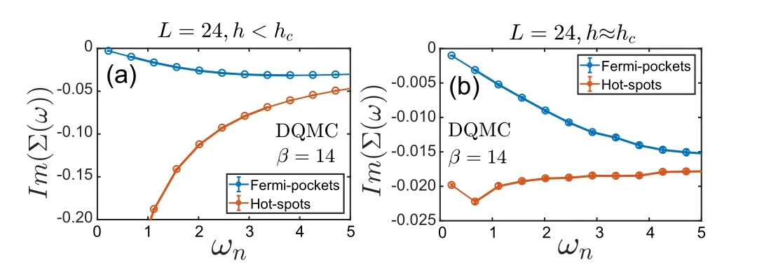
2.4. Bosonic dynamics

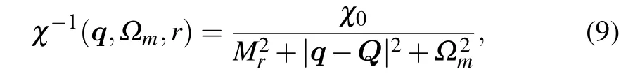
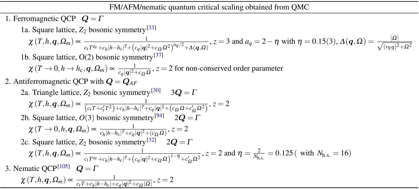
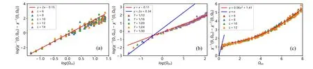
3. Yukawa–Sachdev–Ye–Kitaev model
3.1. Spin-1/2 Yukawa-SYK model and its phase diagram

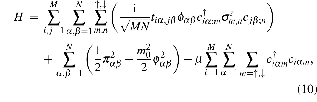
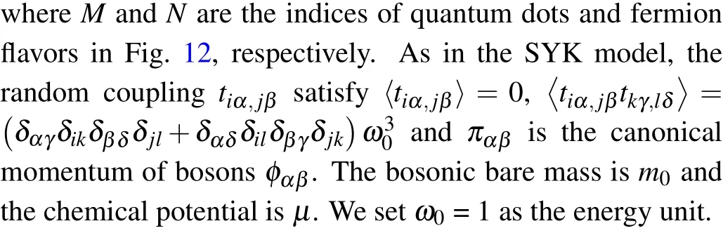


3.2. Normal-state results at N,M →∞
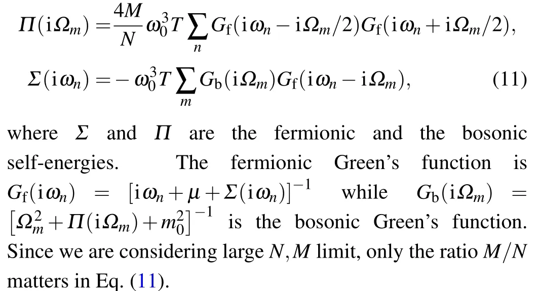
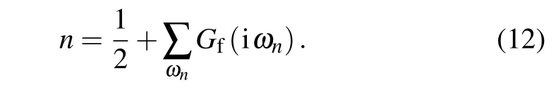

3.3. The nFL Green’s functions
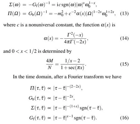

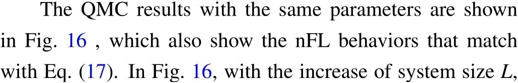

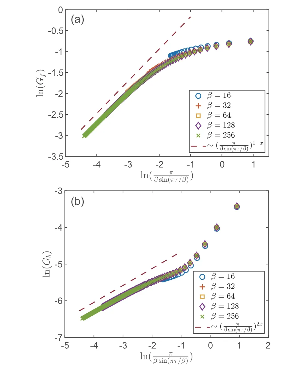


3.4. Self-tuned quantum criticality

3.5. Superconductivity emerging from nFL


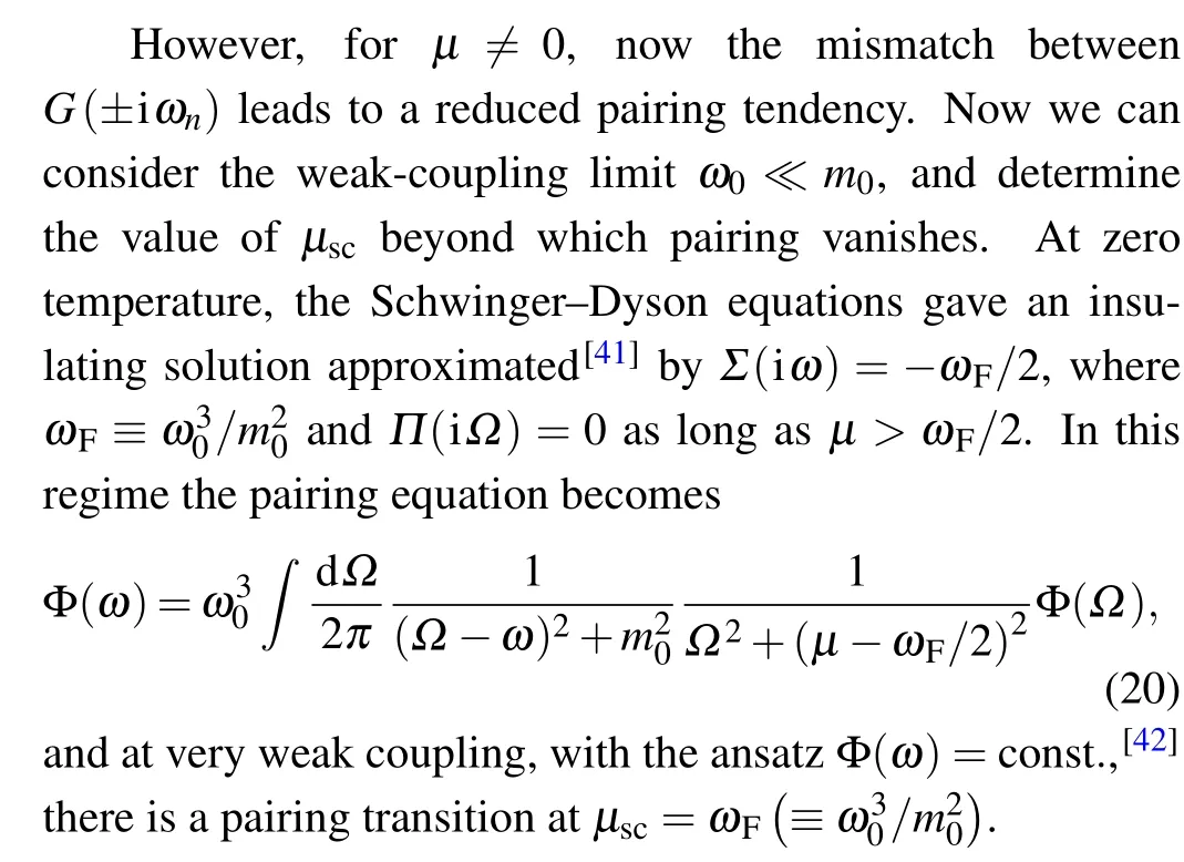

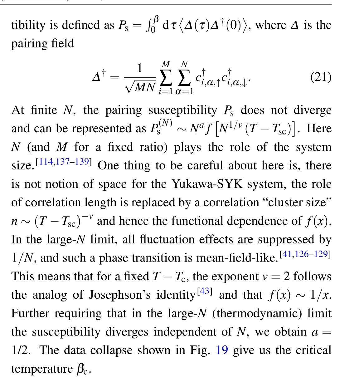

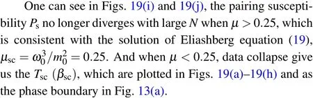
3.6. Planckian metals,spin glass and open questions

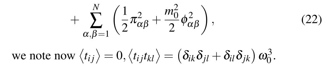
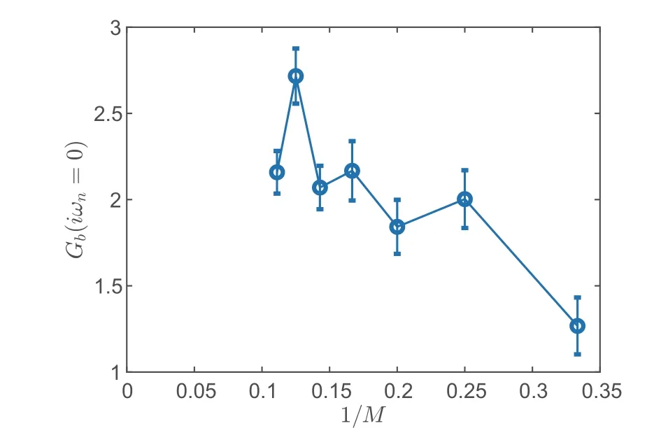

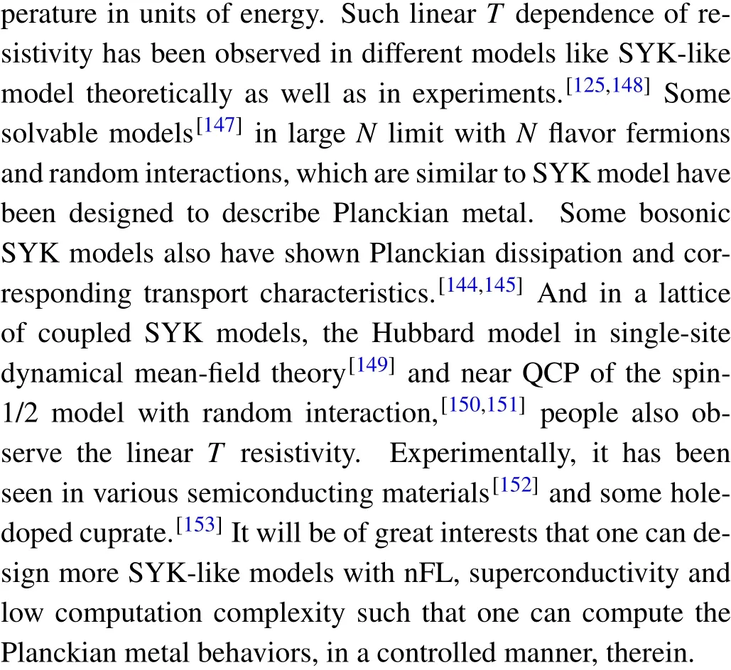
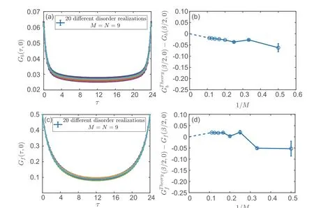
4. Quantum Moire´ lattice models and their computation
4.1. Real-space lattice models


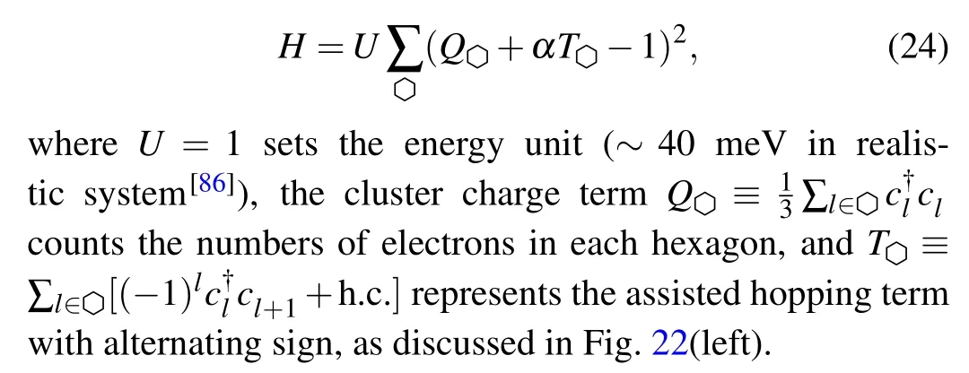

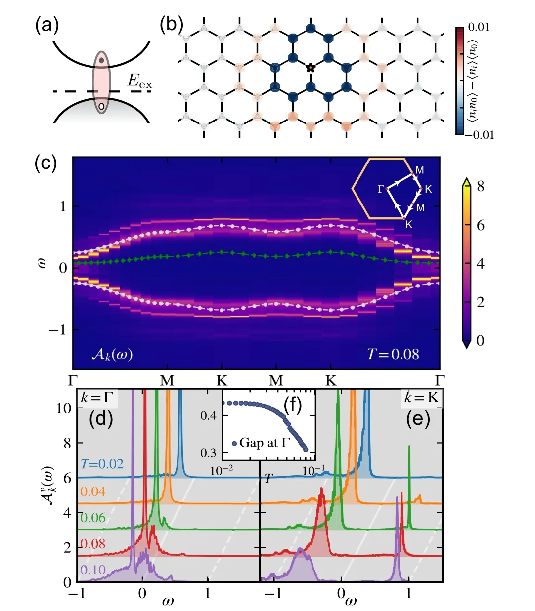
4.2. Momentum-space models and quantum Monte Carlo method


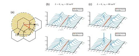
4.3. Dynamical and thermodynamic signatures of the flatband correlations

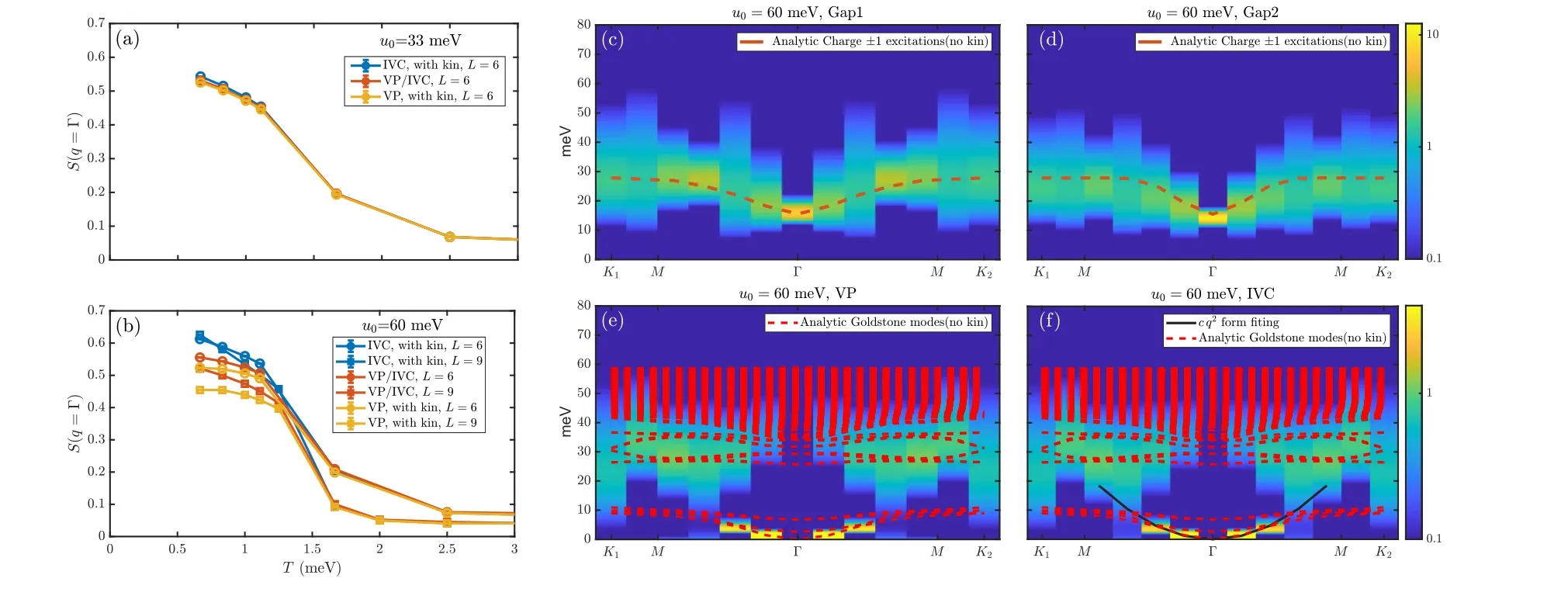
4.4. Symmetry,pairing mechanism and superconductivity
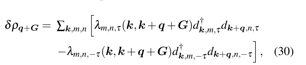
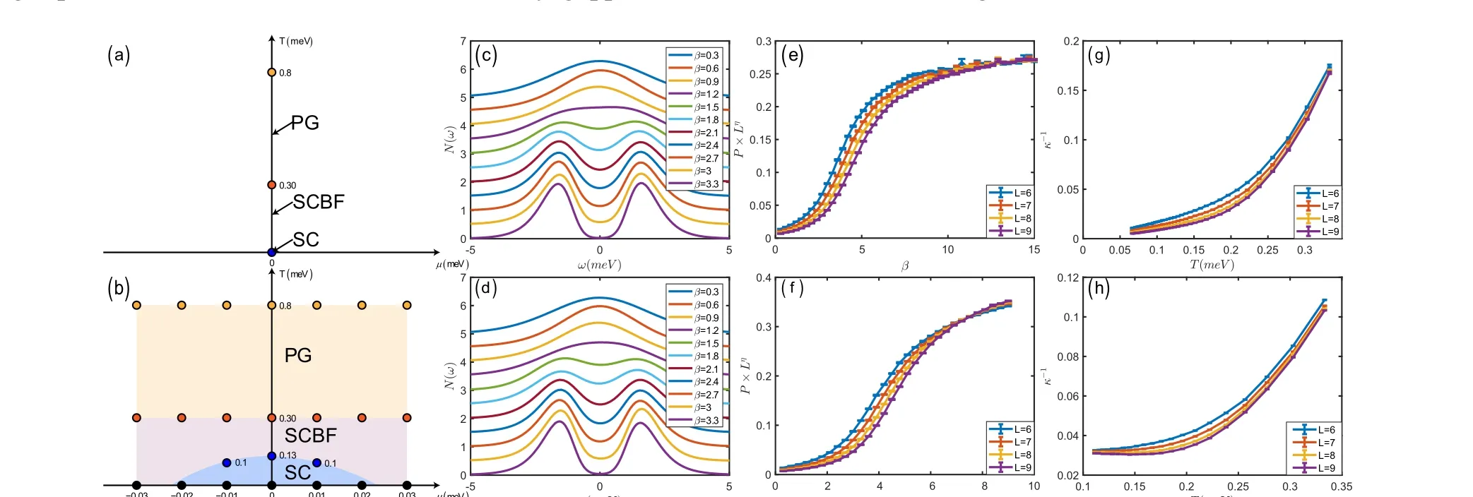

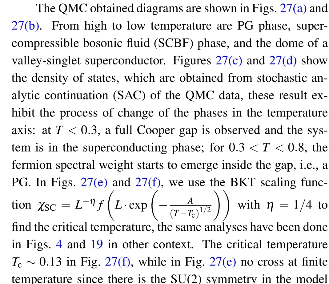
5. Discussion
杂志排行

Chinese Physics B的其它文章
- Editorial:Celebrating the 30 Wonderful Year Journey of Chinese Physics B
- Attosecond spectroscopy for filming the ultrafast movies of atoms,molecules and solids
- Advances of phononics in 20122022
- Molecular beam epitaxy growth of quantum devices
- Single-molecular methodologies for the physical biology of protein machines
- Research progress of Pt and Pt-based cathode electrocatalysts for proton-exchange membrane fuel cells