Jia-Zhen Xu (许家祯), Qi-Hao Cao (曹祺豪) and Chao-Qing Dai (戴朝卿)

Zhejiang A&F University, Lin’an, Zhejiang 311300, China

Abstract The fractional quadric-cubic coupled nonlinear Schrödinger equation is concerned, and vector symmetric and antisymmetric soliton solutions are obtained by the square operator method.The relationship between the Lévy index and the amplitudes of vector symmetric and antisymmetric solitons is investigated.Two components of vector symmetric and antisymmetric solitons show a positive and negative trend with the Lévy index, respectively.The stability intervals of these solitons and the propagation constants corresponding to the maximum and minimum instability growth rates are studied.Results indicate that vector symmetric solitons are more stable and have better interference resistance than vector antisymmetric solitons.

Keywords: fractional quadric-cubic coupled nonlinear Schrödinger equation, vector symmetric solitons, vector antisymmetric solitons, stability

1.Introduction

The study of solitons is of great theoretical and practical importance.In the medium, they are formed because the balance between dispersion and nonlinear effects is subtle.Ren et al proved that an extended mKdV equation is a CRE solvable system[1].Li et al proposed that the electromagnetically induced transparency excites rogue waves, breathers and solitons [2].Wang et al also studied the influence of higher-order nonlinear effects on optical solitons of the complex Swift–Hohenberg model in the mode-locked fiber laser [3].

The nonlinear Schrödinger equation (NLSE) [4, 5] is widely applied in mathematical and physical research.It can be used to describe the water wave model,also to simulate the propagation of light pulses.The NLSE is the basic equation to study the properties of optical solitons, which can describe optical pulses propagating in nonlinear media.A typical NLSE only contains the cubic nonlinear term.In quantum mechanics,ψcan represent the condensed wave function of a weakly interacting non-ideal bosonic gas, while in the classical fluctuation sense,ψcan represent the modulated wave amplitude of deep water surface waves, Langmuir plasma waves and ultrashort light pulses in Kerr media.The fractional Schrödinger equation contains the Laplace operator with Lévy index of1＜α≤2.Longhi reported that the simulation of the fractional Schrödinger equation can be realized by using the resonant cavity in the field of optics,and the Fourier transformation can be realized by phase mask,which can effectively improve the application scope of the nonlinear Schrödinger equation [6].Huang et al firstly proposed the nonlinear fractional Schrödinger equation in the context of optically harmonic lattice and studied the soliton properties in Kerr media [7].Zhang et al discussed the transmission of optical beams in the fractional Schrödinger equation with harmonic potential in the one- and twodimensional cases[8].Zhang et al studied the propagation of one- and two-dimensional Gaussian beams in the fractional Schrödinger equation without potential[9].Feng et al studied the propagation dynamics of the beam in the presence and absence of the beam’s chirp[10].Wang et al found analytical fractional solitons for the space-time fractional Fokas–Lenells equation [11].

In nonlinear optics, the coupled nonlinear Schrödinger equation(CNLSE)is able to describe the interaction between modes in a wider range of physical situations than the single equation [12].In the early studies of coupled nonlinear systems, Manakov et al found that the system is productible when the coefficient of the cross-phase modulation is equal to that of the self-phase modulation by the cross-phase modulation [13–15].Wang et al studied CNLSE using the generalized DT method to obtain the dynamical states of second-order local waves [16].Coupled systems containing higher-order nonlinear effects generate many physical phenomena, such as the self-steepening effects [17–19] and Raman scattering[20–23].In recent years,Song et al studied three spiraling anomalous vortex beam (AVB) arrays with different propagation states are studied[24],and the evolution of Gaussian-shaped soliton clusters in strongly nonlocal nonlinear media [25].

However, the system of CNLSE containing quadriccubic competing nonlinear effects has not been investigated and little is known about the physical mechanisms involved.In this paper, we generalize the NLSE [26] to fractional quadric-cubic CNLSE (FQCCNLSE).Here we add a quadratic nonlinear term to explore the competition between quadratic and cubic nonlinearities and the effect of both on solitons.Through the add of the competition between the quadratic and cubic nonlinear terms in the coupled model,we are able to have applications in a wider range of physical contexts to better achieve stable transmission of solitons.

In section 2, we discuss the modeling of the FQCCNLSE.In section 3, we solve the two components of coupled symmetric and anti-symmetric solitons and perform stability analysis.In section 4 we investigate the relationship between the propagation constants of the two components of the coupled symmetric and anti-symmetric solitons and the maximum unstable growth rate.In section 5,we conclude this paper.

2.Model

The FQCCNLSE can be written as

where functionsψ1,ψ2are smooth wave envelope functions containing two spatial variablesξ,ζ.The first term of the equation can represent the wave transmission,the second item refers to the dispersion effect, the third term is the refractive index modulation term,the fourth term donates the Kerr term,and the last terms represent nonlinear effect.When we take the value of α to be 2, equation (1) will become an integerorder quadric-cubic CNLSE describing some nonlinear dynamics.If equation(1)is decoupled with settingψ2= 0,it becomes the single equation in [26].

Here we take the potential function as [27]

By takingψ1(ζ,ξ) =ψ1(ξ) eiβζ,ψ2(ζ,ξ) =ψ2(ξ)eiβζinto equation (1), we obtain

3.Vector solitons and their stability analysis

First, by the square operator method [26], we solve equation (1) and obtain the soliton solution.Here, we setλ= -1 andσ= 1 with representing the self-defocusing quadratic nonlinearity and self-focusing Kerr nonlinearity.We set the parameter V0of the potential function as 1.3, the single-peak widthω0as 1.4, the distance between the two peaksξ0as 1.5, and the Lévy indexαas in the range of 1.3–1.9[19].We set the initial propagation constantβto 0.8,then we can get the symmetric and antisymmetric vector soliton solutions of equation (1) numerically in figure 1.

From figures 1(a) and (b), we can see that the amplitude of the vector symmetric soliton (particularly pronounced at the top) grows with the add of the Lévy index.From figures 1(e) and (f), it can be seen that the peak height of the vector antisymmetric soliton reduces with the increasing Lévy index.It can be simply seen that the Lévy index has different effects on vector symmetric solitons and vector antisymmetric solitons, in terms of waveform and amplitude.For vector symmetric solitons, the Lévy index shows a positive trend with the soliton amplitude, while for vector antisymmetric solitons, the Lévy index shows a negative trend with the soliton amplitude.

Then we analyze the two components of the vector symmetric soliton and vector antisymmetric soliton, we add tiny perturbationsμ(ξ) andv(ξ)to the stable solutionsψ1(ξ)andψ2(ξ)and obtain the following form

whereμ(ξ) andv(ξ)denote the amount of small perturbations,*denotes its conjugate form, andλrepresents the growth rate of instability.By deriving the calculation, we get the eigenvalue problem as

with the eigenvalueδforψ1(ζ,ξ)as

and forψ2(ζ,ξ)as

For the linear stable spectrum,we can obtain the unstable growth rate of the soliton solution according to the real part of δ.In the numerical simulation, the real part of the eigenvalue is inversely related to the stability of the soliton solution.When the real part ofδis 0, the linear stability of soliton is better.

We simulated the evolution of solitons for the 5% perturbation case using a fast Fourier algorithm.From the illustrations in figures 1(c), (d), we can see that maximum unstable growth rate in the linear stability spectrum are all 0.It indicates that the vector symmetric solitons are stable,which can be verified by the evolution diagram of figures 1(c),(d).The real and imaginary parts ofδare denoted byδRandδI, respectively.The evolutionary shape of the vector symmetric soliton remains unchanged during the evolution, and only minor fluctuations occur due to the presence of 5% white noise interference.In figures 1(g), (h), we can see that the maximum unstable growth rate of the eigenvalue becomes nonzero, indicating the poor stability performance of vector antisymmetric solitons.Under the interference of 5%white noise,figures 1(g),(h)show that the evolution of vector antisymmetric solitons is unstable and their shapes of solitons exhibit a spiky shape, which is in accordance with the results of the stability analysis.

Figure 1.(a),(b)Vector symmetric soliton and(e),(f)vector antisymmetric soliton for different Lévy index when the propagation constant β = 0.8.Evolution diagrams of vector symmetric soliton for (c)ψ1 and (d)ψ2 and vector antisymmetric soliton for (g)ψ1 and (h)ψ 2.The illustrations in (a), (b), (e), (f) are enlargements of the top of the soliton, and the insets in (c), (d), (g), (h) show the corresponding linear stability analysis.Parameters are V0 =1.3,ω 0 = 1.4,ξ 0 = 1.5,α =1.3~ 1.9,λ = -1,σ = 1.

Through the above study we can draw conclusions that the solitons with good stability have anti-interference properties,for example,the vector symmetric solitons maintain the same amplitude and shape under the interference of 5%white noise, and only some small oscillations occur.However, the waveform and amplitude of unstable solitons vary more,especially in their tails.This indicates that the stable solitons can play a better anti-interference role.

4.The stability interval of vector solitons

In the following we investigate the connection between the propagation constant β and real partδRfor vector symmetric and antisymmetric solitons, as shown in figure 2.

Figure 2.The connection between the propagation constant β and real partδR for vector symmetric solitons with(a)ψ1 and(b)ψ2 and vector antisymmetric solitons with(c)ψ1(b)ψ 2. β ranges from 0.5 to 1.8 in steps of 0.1 in(a),(b),and from 0.4 to 1.8 in steps of 0.05 in(c),(d).Parameters are V0 =1.3,ω 0 = 1.4,ξ 0 = 1.5,α = 1.7,λ = -1,σ = 1.

Figures 2(a),(b)reflect the connection betweenδRandβfor two componentsψ1andψ2of vector symmetric solitons,respectively.In figure 2(a), when the value ofβlies in [0.5,1.6],the maximum unstable growth rate is bigger than 0,and it can be seen that the componentψ1is unstable in this interval.When the value ofβis located at [1.6, 1.8],δRbecomes 0, denoting that the componentψ1is stable in this interval.In figure 2(b),it can be also seen that the componentψ2is unstable in the interval [0.5, 1.5] and stable in the interval [1.5, 1.8].To further investigate the accuracy of this result, these points with the maximum and minimum propagation constants for componentsψ1andψ2are chosen for the numerical evolution and stability analysis, respectively.In figure 2(a), we choose the cases of minimumβ= 1.4 and maximumβ= 1.6.From figure 3(a), we know that whenβ=1.4,the value ofδRfor the componentψ1is bigger than 0 and vector soliton solutions are unstable.This result is also verified by this case in figure 3(c).Whenβ=1.6,the real part of the eigenvalue for the componentψ1is equal to 0 as known from figure 3(e), and soliton solution for this component is stable.This case is also verified in figure 3(g).Similarly, we verify the same case for componentψ2by choosing the maximum propagation constantβ= 0.9 and the minimum propagation constantβ= 1.5, respectively.Whenβ= 0.9,the value ofδRfor the componentψ2becomes nonzero,denoting that soliton solution for this component is unstable,which is also verified in figures 3(b), (d).Whenβ= 1.5, the value ofδRfor the componentψ2is equal to 0 and soliton solution for this component is stable,which is also verified in figures 3(g), (h).

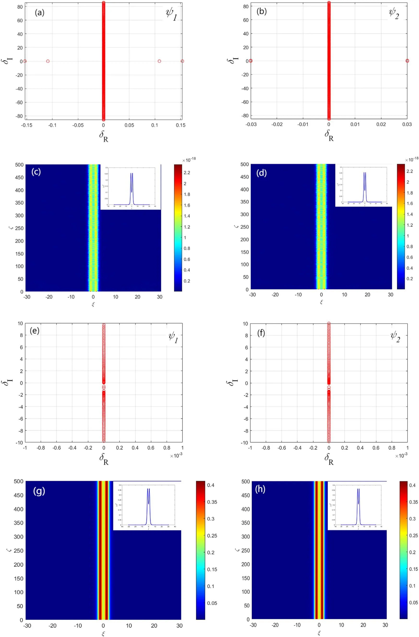
Figure 3.The linear characteristic spectra of vector symmetric solitons for the componentψ1 with (a) β = 1.4 and (e) β = 1.6 and the componentψ2 with(b)β =0.9 and(f)β =1.5.(c),(g),(d),(h)Numerical simulation plots corresponding to(a),(e),(b),(f).The insets in(c),(g), (d), (h) represent the soliton shape at ζ = 250 during the numerical simulation.The parameters are the same as in figure 1.

For two componentsψ1andψ2of vector antisymmetric solitons in figure 2(c),the value ofδRfor the componentψ1is bigger than 0 whenβlies between [0.4, 1.05], indicating the instability of soliton solution, and the value ofδRfor the componentψ1is equal to 0 whenβlies in [1.05, 1.8], indicating that the soliton solution is stable.In figure 2(d), whenβlies between[0.4,1.05],the value ofδRfor the componentψ2is bigger than 0, indicating that the soliton solution is unstable,and when theβlies in[1.05,1.8],the value ofδRfor the componentψ2is nearly equal to 0, indicating that the soliton solution is stable.We choose these points with the maximum propagation constantβ=0.65 forψ1andβ=0.75 forψ2,and minimum propagation constantβ= 1.05 for the stability analysis and numerical evolution.The validation results are exhibited in figure 4.

Figures 4(a),(e)exhibit the linear characteristic spectrum of the componentψ1for vector antisymmetric solitons when the propagation constantβis 0.65 and 1.05, respectively.From figures 4(c), (g), it can be seen that the soliton has obvious oscillations and presents an unstable state whenβ= 0.65, and the soliton is stable whenβ= 1.05.Figures 4(b), (f) shows the linear characteristic spectrum of the componentψ2for vector antisymmetric solitons when the propagation constantβis 0.75 and 1.05, respectively.It can be seen from figures 4(d),(h)that the oscillation of the soliton is obvious whenβ= 0.75, and the soliton propagation is stable whenβ= 1.05.

Figure 4.The linear characteristic spectra of vector antisymmetric solitons for the componentψ1 with(a)β =0.65 and(e)β =1.05 and the componentψ2 with(b)β =0.75 and(f)β =1.05.(c),(g),(d),(h)Numerical simulation plots corresponding to(a),(e),(b),(f).The insets in(c), (g), (d), (h) represent the soliton shape at ζ = 250 during the numerical simulation.The parameters are the same as in figure 1.

5.Summary

In this paper, we study the FQCCNLSE and obtain vector soliton solutions by the square operator method.Moreover,we investigate the relationship between the Lévy index and the amplitudes of the vector symmetric and antisymmetric solitons.Two components of vector symmetric and antisymmetric solitons show a positive and negative trend with the Lévy index, respectively.We also give the stability intervals of these solitons and the propagation constants at the maximum and minimum instability growth rates, and finally find that the stable solitons with good anti-interference are important for stable transmission of optical soliton communication in fiber, and the research in this paper effectively promotes the development of vector solitons in the field of nonlinear optics.

Acknowledgments

This work is supported by Zhejiang Provincial Natural Science Foundation of China (No.LR20A050001), National Natural Science Foundation of China (No.12075210), and the Scientific Research and Developed Fund of Zhejiang A&F University (Grant No.2021FR0009).