Sibel Tarla, Karmina K Ali,2, Resat Yilmazer and M S Osman

1 Department of Mathematics, Faculty of Science, Firat University, Elazig, Turkey

2 Department of Mathematics, Faculty of Science, University of Zakho, Zakho, Iraq

3 Department of Mathematics, Faculty of Science, Cairo University, Giza 12613, Egypt

Abstract This study investigates the perturbed Chen–Lee–Liu model that represents the propagation of an optical pulse in plasma and optical fiber.The generalized exponential rational function method is used for this purpose.As a result, we obtain some non-trivial solutions such as the optical singular, periodic, hyperbolic, exponential, trigonometric soliton solutions.We aim to express the pulse propagation of the generated solutions,by taking specific values for the free parameters existed in the obtained solutions.The obtained results show that the generalized exponential rational function technique is applicable, simple and effective to get the solutions of nonlinear engineering and physical problems.Moreover, the acquired solutions display rich dynamical evolutions that are important in practical applications.

Keywords: perturbed Chen–Lee–Liu model, generalized exponential rational function method,analytical solutions

1.Introduction

Researchers have taken great attention to study nonlinear phenomena.Nonlinear partial differential equations (NPDEs)appear in applied mathematics and engineering research areas with various applications.Several goals of applied mathematics are presented to identify and explain exact solutions for NPDEs [1–8].Numerous NPDEs such as the Sawada–Kotera equation[9–11],the Gilson–Pickering model[12,13],the Fokas–Lenells model [14–16], the Hirota equation[17, 18], the Sasa–Satsuma equation [19–21], and others[22–31] have been discussed and analyzed in different branches of science

The perturbed CLL model is given by [32]:

whereγis the inter-modal dispersion coefficient,μsymbolizes the coefficient of self-steepening for short pulses, andδis the coefficient of nonlinear dispersion.Additionally,αis the coefficient of the velocity dispersion andβis the coefficient of nonlinearity.Here, equation (1) is studied whenm=1

The main object of this article is to study and analyze equation (2) by finding a variety of solutions via the GERFM for the perturbed CLL model that represents the propagation of an optical pulse in plasma and optical fiber.Recently, the field of applications of this equation has become an important part of plasma physics.Previously this equation has been investigated by many researchers.Houwe et al [33] show the chirped and the corresponding chirp with their stability for the CLL model.Biswas has obtained soliton solutions by using semi-inverse variational principle[34].Akinyemi and others studied the CLL model with the help of the Jacobi elliptic functions [35].Kudryashov found general solutions by using different methods with the elliptic function approach [36].Apart from this, the Sardar subequation technique was utilized to obtain solitary wave solutions for this equation [37], and numerous studies have been done for the CLL model [38–40].In this study, we examine this model via the generalized exponential rational function method (GERFM).This method is presented by Ghanbari and others to study different partial differential equations[41,42].Furthermore,Ghanbari and Aguilar used this approach to find some novel solutions of the Radhakrishnan–Kundu–Lakshmanan equation withβ-conformable time derivative [43].

This study is organized as follows; introduction is given in section 1.In section 2, we focused on presenting the GERFM.In section 3,we established and studied a variety of exact solutions for the perturbed CLL model by applying the GERFM.The conclusion and the physical interpretations of this study are presented in section 4.

2.Outline of GERFM

In this section,the GERFM is explained in the following manner:

Step 1:Consider the general form of a nonlinear partial differential as:

whereQis a polynomial function inψ(x,t)and its partial derivatives.Suppose that the wave transformation takes the form:

whereP(η) is the amplitude,kis the wave number,wis the frequency,θis the phase constant,andx-htis the traveling coordinate.Equation (3) becomes a nonlinear ordinary differential equation with the use of equation (4) and written as:

Step 2:The solitary wave solutions of equation(5)have the form:

where

herern,sn(1 ≤n≤ 4)are real/ complex constants,A0,AK,BKare constants to be determined, andnwill be determined by the known balance principle.

Step 3:Substituting equation (6) into equation (5), we get a system of polynomials inφ(η).By equating the same order terms, we obtain an algebraic system of equations.By using any suitable computer software, we solve this system and determine the values ofA0,AK,BK.Thus, we can easily obtain non-trivial exact solutions of equation (5).

Step 4:Putting non-trivial solutions obtained from Step 3 into (6), we attain the exact soliton solutions of equation (2).

3.Applications

In this portion,we apply the GERFM to equation(2).Firstly,inserting equation (4) into equation (2) yields

The real part of equation (8) is given by

and the imaginary part has the form

Set the coefficients of the components of the imaginary part equal zero, we geth= -2kα-γ,andβ= 3μ+2δ.Considering these constraints in equation (9), we get

By using the balance principle, we getn=1.Also, we user=[r1,r2,r3,r4]ands=[s1,s2,s3,s4]notation.Considering equations(6)and(7),we may express the solution of equation (11) as follow:

Family 1:Forr= [- 2, -1 , 1, 1],s=[0 , 1, 0, 1],we get

Taking into account equations(12)and(13)and by direct substitution in equation (4), we get

Consideringh= - 2kα-γ,the exact solution of equation (2) reads

This is corresponding to optical exponential solutions.

Consideringh= -2k α-γyields the exact solution of equation (2) as

Equation (15) represents optical exponential solutions.

Consideringh= -2kα-γ,we reach the exact solution of equation (2) as

This is corresponding to optical trigonometric solutions under conditionsα＞0,k(δ+μ)＜0.

Taking into account equation (12), equation (16), and these values in equation (4), we get

Consideringh= -2kα-γ,we get the exact solution of equation (2) as follows

Equation (18) is corresponding to the optical trigonometric solutions under conditionsα＞0,k(δ+μ)＜0.

Family 3:In this groupr=[2 , 0, 1, 1],s= [-1 , 0, 1, - 1],we get

Case 1:Whenand.

Taking into account equation (12), equation (19), and these values in equation (4), we obtain

Consideringh= -2kα-γ,we get the exact solution of equation (2) as follows

This is corresponding to the optical hyperbolic solutions under conditionsα＞0,k(δ+μ)＜0.

Family 4:Forr= [ -1 , 1, 1, 1],s= [1, -1 , 1, - 1],we get

Case 1:Whenand

Taking into account equation (12), equation (21), and these values in equation (4), we have

Consideringh= -2kα-γ,the exact solution of equation (2) takes the form

This is corresponding to the optical singular soliton solutions under conditionsα＞0,k(δ+μ)＜0.

In figure (4),the amplitude of the solution given is very high in the medium through which the wave is propagated,thus this singular periodic wave is a shock wave.

Family 5:Usingr= [i , -i , 1, 1],s= [i , -i , i, - i],we get

Taking into account equation (12), equation (23), and these values in equation (4), we obtain

Consideringh= -2kα-γ,the exact solution of equation (2) takes the form

This is corresponding to the optical periodic soliton solutions under conditionsα＞0,k(δ+μ)＜0.

Case 2:WhenA0=0,A1=0,and.

Taking into account equation (12), equation (23) and these values in equation (4), we get

Consideringh= -2kα-γ,the exact solution of equation (2) is given by

Equation (25) is corresponding to the optical periodic soliton solutions under conditionsα＞0,k(δ+μ)＜0.

4.Conclusion

Herein, we have divided our results into two main parts as follows:

4.1.Overview

The current work recovered a variety of optical soliton solutions with different wave structures for the perturbed CLL model is obtained via the GERFM.According to the suitable choice of the self-steepening short pulsesμand the nonlinear dispersion coefficientδ, the obtained solutions are classified into optical singular, periodic, hyperbolic, exponential, and trigonometric soliton solutions.Furthermore, the physical meaning of these solutions is graphically investigated through 2D-and 3D-plots.To the best of our knowledge,these results were obtained for the first time for this model.This kind of study is helpful for a physician in planning and decisionmaking for the treatment of optical pulse in plasma and optical fibers.

4.2.The physical interpretation

In figures 1–5, as changing the values ofμandδ, the rise steepening of the wave will change.For different values of the parameterα, as an example, the velocity distribution of the wave will be changed as seen in figure 3.In figure 4,when the value ofwis increased,the wavelength is decreased.This feature is also observed in figures 1–5.In summary, the obtained solutions are classified into the following categories:equations (14) and (15) represent optical exponential solutions, equations (17) and (18) investigate optical trigonometric solutions, equation (20) represents an optical hyperbolic solutions, equation (22) shows an optical singular soliton solution,and finally equations(24)and(25)introduce optical periodic soliton solutions.

Figure 1.Optical exponential solutions of equation (14) for the values of A1 = 0.2,w = 2,k =0.1, δ = 0.1,μ = 0.2,and θ =1.3.

Figure 2.Optical trigonometric solutions of equation (17) for the values ofα = 2,k= -1, θ = 0.5,μ = 0.6,δ = 0.4,and w =0.2.

Figure 3.Optical hyperbolic solutions of equation (20) whereα =1, w =1, k= -2,δ =2,μ =1, andθ =2.

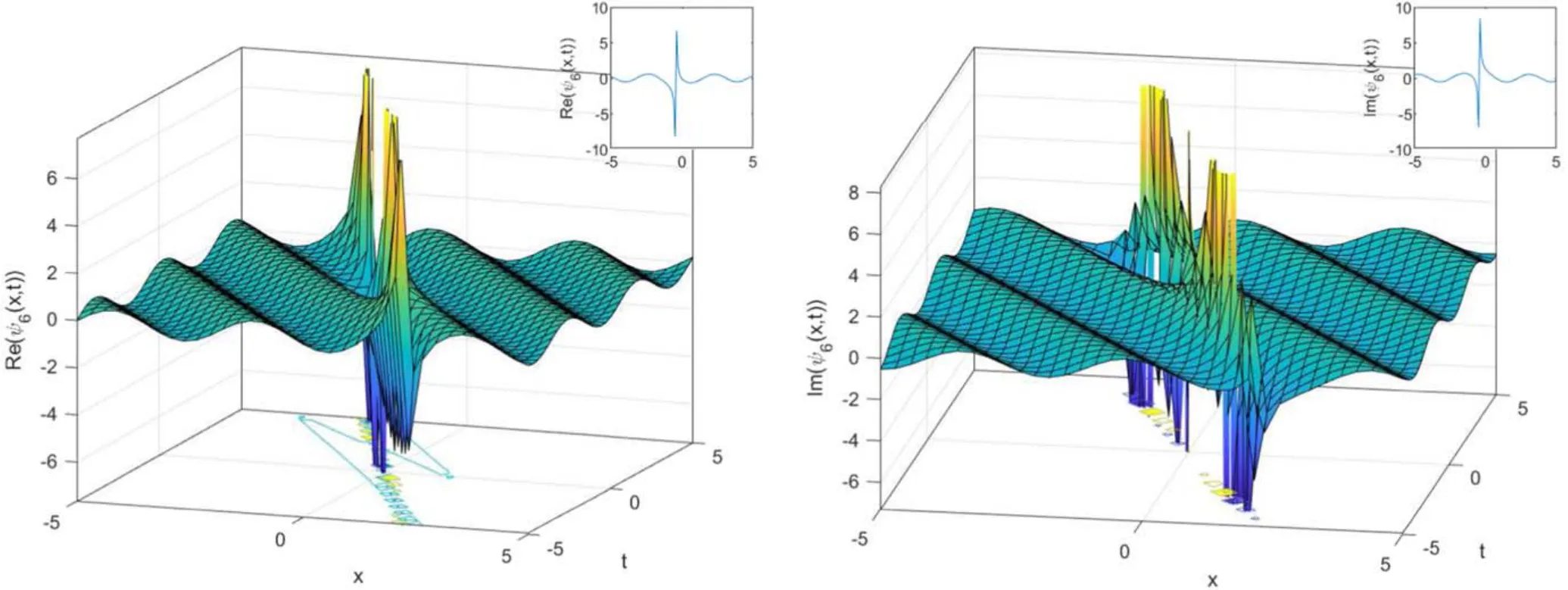
Figure 4 Optical singular soliton solutions of equation (22) using α = 0.3,w =1.5,k= -2, δ = 0.5,μ = 0.02,and θ =0.2.

Figure 5.Optical periodic soliton solutions of equation (24) for the values of α = 1.7,w = 2,k =2, δ = -1 .5,μ = -0 .1,and θ =0.02.

Acknowledgments

Author Sibel Tarla is a 100 2000the council of Higher Education(CoHE)PhD scholar in computational science and engineering sub-division.

ORCID iDs