Xueyi Guan(管学义)， Rongjun Cheng(程荣军)， and Hongxia Ge(葛红霞)

Faculty of Maritime and Transportation，Ningbo University，Ningbo 315211，China

Keywords: visual angle，bifurcation analysis，anticipated time，stabilizing driving behavior，TDGL and mKdV equations

1. Introduction

In recent years， the demand for transportation has maintained a continuous growth， which has brought huge challenges to the smooth traffic and traffic safety. Facing the traffic problems，numerous of scholars proposed a series of traffic flow models to explain the complex traffic phenomena. These models[1–9]mainly model the traffic flow from three modules:macroscopic，microscopic and mesoscopic. For example，Sunet al.[1]proposed a car-following model， one of the microscopic models of vehicular traffic， which is concentrating on individual vehicles，and studying the characteristics of the following vehicles in the entire fleet by studying the influence of the changes in the movement state of the leading vehicle on the following vehicles， meanwhile the theoretical analysis and simulation of the improved model not only can provide deep exploring into the properties of the model but also help in better understanding the complex phenomena observed in real traffic fields. In addition，we can also subdivide these models into the car-following models (e.g.， Sunet al.，[1]Geet al.[2]and Jianget al.[3])， the cellular automation models (Tianet al.[4])， the gas kinetic models (Nagataniet al.[5])， the hydrodynamic lattice models (Redhuet al.[6]and Changet al.[7])and the continuum models(Chenget al.[8]and Zhaiet al.[9])according to different modeling theories. Bifurcation， as an important research content of non-linear science，mainly studies the instability of the system solution caused by parameter changes and the changing behavior of the number of solutions.Studying the bifurcation in traffic flow will have important theoretical implications in analyzing traffic phenomena， traffic modeling，traffic control，etc.

Facing numerous of traffic congestions， a number of mathematical models have been proposed to demonstrate the car-following behavior under various conditions with the development of urban transportation. Generally speaking，these models are mostly based on the stimulus-response framework，which was put forward at the General Motors research laboratories (Chandleret al.[10]and Gaziset al.[11]) at the first time. According to the framework，each driver responds when giving a stimulus. And the relationship between response and stimulus is as follows:

In the framework， the stimulus could be mainly divided into four aspects: driver’s behavior factors， vehicle factors， road factors and other factors. However， when it comes to carfollowing model equation，the stimulus could be related to the location of a large number of cars or their speed， or maybe some other coefficient. The reaction which demonstrates the propulsion of follower has been transformed into vehicle’s speeds or accelerations. In different forms of car-following models， the reason for the different forms of vehicle motion equations lies in the different hypotheses of stimulus properties. The stimulus is probably composed of the speed， the speed difference between two consecutive vehicles，the headway， etc. Following are some classic car-following models that consider different stimulus.

Gazis–Herman–Rothery (GHR)[11]car-following model is perhaps the most recognized model in the research of traffic flow， which is the foundation of the car-following model proposed by Hermanet al.[12]and Yanget al.，[13]displayed as

whereλis the sensitivity of the relative velocity， Δvn(t-τ)represents the relative velocity of thenth car at timet-τ，τis reaction time of driver，in addition，andλhas some functional forms as follows:

where Δxn(t)represents distance between two consecutive vehicles， Δxcritical(t) is the threshold value obtained from actual data analysis，vn(t)represents the velocity ofnth vehicle，whileA，A1andA2are constant. Moreover， Lee[16]believed that drivers make decisions relying on a period of stimulation rather than a transient stimulus，and for the reason he proposed an improved GM model with considering driver’s memory，which is the foundation of the extended car-following model considering driver’s memory and jerk proposed by Jinet al.[17]

For whether Chandleret al.[10]or Gaziset al.[11]mentioned earlier， they all assumed that both cars are driving at the same speed and the headway is acceptable， but this is not consistent with the actual situation. To overcome this shortcoming，Newell[18]proposed a nonlinear car-following model by using the headway as a stimulus， and Helly[19]assumed that every driver will adjust the following distance to a desired distance according to his driving characteristics， and drivers strive to minimize the relative speed along with the distance between the actual headway and the required headway，which is defined as

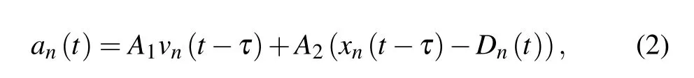
whereDn(t) is driver’s desired following distance. In view of the earlier work， Helly[19]calculated the final calibration results whereτ=0.5 s，A1=0.5 s-1，A2=0.125 s-2， andDn(t)=20+vn(t-0.5). And Helly’s improvement also laid the foundation for the innovation of Koshiet al.[20]and Xinget al.[21]For example， Koshiet al.[20]combined Helly’s model with GHR’s model and did a nonlinear extension， but it still has some shortcomings in horizontal curvature effect.

Then in 1995， Bando[22]proposed the optimal velocity(OV) model， which describes some nonlinear phenomenon and car-following behavior in traffic， and the specific expression shows as following:

whereαdonates the coefficient of sensitivity andVrepresents the optimal velocity that drivers prefer based on the condition of the headway.

Optimal velocity model can reflect some actual traffic flow characteristics such as the disappearance of stability of continuous traffic flow， the queuing of the traffic and the entire process from the generation to the elimination of traffic congestion very well， but when facing high acceleration values， it has certain defects. Helbing and Tilch[23]compiled a large amount of empirical data to overcome this shortcoming and proposed a generalized force (GF) model. The same as GHR model， GF model considered the effect of relative speed， too， but the model ignored the situation where the velocity of the follower is equal to or less than the velocity of the leader. Then， Jianget al.[24]proposed the full velocity difference(FVD)model，which considers the positive relative velocity. Therefore， the FVD model can describe the actual traffic flow better compared to the OV and GF models during the car-following process. Its formula reads

in whichV(θn(t))represents the relative velocity andλis its sensitivity coefficient. In 2019， Yanet al.[25]improved the FVD by taking the optimal velocity difference and the electronic throttle angle difference of the preceding vehicle into account so as to explain the current complex traffic situation.

In the model， driver’s response is mainly coming from the stimulus of both speed difference and headway. However，since Michaels[26]introduced psychology-related theories into the car-following model for the first time，a series of follow-up studies (e.g.， Winsum[27]) showed that psychological characteristics are indeed related to the stability of traffic flow. Its main performance is that visual angle can be used to replace headway together with angular velocity， which can be used to replace speed difference in some engineering car-following models. Therefore，Andersen and Sauer[28]proposed the driving by visual angle (DVA) model by taking visual angle into account based on Helly’s[19]model.

Combined the FVD with DVA model，Jinet al.[29]developed the visual angle model(VAM)which takes both positive velocity difference and visual angle into account defined as

whereV(θn(t)) represents the optimal velocity according to the visual angle of the driver， andθn(t) represents visual angle observed by the driver of carnat timet，as shown in Fig.1.

As we all know， car-following behavior is a humanrelated process， and inserting visual angle into the FVD can access to 3D parameters information directly， which is closer to reality. However， in order to reduce gasoline consumption and stop-and-go while driving，many drivers always try to keep the vehicle as smooth as possible， which means that drivers will control the headway far enough to accelerate， but in order to avoid the repeated deceleration， the driver may drive smoothly at the original speed rather than accelerating. Therefore， in addition to the influence of visual angle and relative speed，driver’s stabilizing driving behavior can also affect the driving behavior， and for this reason， based on the VAM， in this paper we propose an improved car-following model by taking the effect of visual angle，anticipated time and driver’s stabilizing driving behavior into account.

Bifurcation is defined as the process in which the nonlinear dynamic parameters of the system continuously change and reach a certain critical point，which causes the global nature of the system to change. In 1978， Huilgol[30]firstly introduced the bifurcation theory to the nonlinear dynamics of vehicle systems，which aroused the enthusiasm of traffic scholars around the world to study the stability of vehicle systems.With the continuous development of bifurcation analysis theory，Igarashiet al.[31]and Oroszet al.[32]selected different optimal velocity functions to study the bifurcation phenomenon in the OV model，and obtained the similar conclusions，which was later extended to the OVM with a single fixed delay by Yamamotoet al.[33]performed Hopf bifurcation analysis for the dissipative system with asymmetric interaction including the OVM. It is generally found that a bifurcation structure is related to the multiple traffic jams via the transitions of emerging clusters(i.e.，traveling waves). In order to further explore the relationship between traffic state and bifurcation，in 2004，Gasseret al.[34]conducted a series of car-following models with bifurcation analyses. They found that the instability of the neutral stable solution increased in optimal velocity models is normally owing to the happen of the Hopf bifurcation.Jinet al.[35]conducted a bifurcation analysis for the FVD model to study the effect of bifurcation behavior on traffic congestion and stability of the system. More recently， Zhanget al.[36]studied the traditional velocity difference model considering time delays. They found that bifurcation happened corresponding to the emergence of traffic congestion in continuous traffic flow. Nowadays，a great progress on traffic flow has been made. However， it is still essential to explore and grasp the nonlinear characteristic of traffic information so as to eliminate the traffic jams.

Through the review of the development of traffic flow theory，we can find that few studies have comprehensively considered the driver’s visual angle，anticipated time and driver’s stable driving behavior to explore the impact of these characteristics on car-following behavior. While the article focuses on three human factors， comprehensively considers the driver’s visual angle， anticipated time and stable driving behavior to explore the impact of driver behavior factors on car-following behavior. Then the influence of various factors on the stability of traffic flow is obtained through the linear， nonlinear analysis and numerical simulation. Finally， the rationality of the improved model is verified by parameter calibration.

The specific contribution of this paper are as follows:

(1)Providing theoretical support for the establishment of intelligent transportation systems. In the process of developing self-driving vehicles，robots can be used to simulate human driving，and the optimal human psycho-physiological characteristics are set during the robot programming，so as to achieve the maximum safety and optimal efficiency of the traffic flow.

(2)Providing references for traffic management systems.In terms of traffic safety， the optimal driver’s psychologicalphysical characteristics obtained from the study can be used as the reference standard to strictly review the driver’s driving qualification.

The following is the framework of the article. First of all，we make an overview of the development of the traffic flow in Section 1.Then we take visual angle，anticipated time and stabilizing driving behavior into account and put forward a new visual angle model in Section 2. In Section 3，the neutral stability curve is carried out through linear stability analysis. In Section 4 we conduct bifurcation analysis for the improved model and study the influence of the three driver’s behavior on Hopf bifurcation. Through the numerical calculation， the time-dependent Ginzburg–Landau (TDGL) equation and the modified Korteweg–de Vries (mKdV) equation are given respectively in Sections 5 and 6. Then in Section 7， parameter calibration and numerical simulations are carried out and numerical results are discussed. Finally， we obtain the conclusions in Section 8.

2. The extended car-following model

All of the previous car-following models are developed based on the ideal state that the driver’s immediate response to traffic conditions is absolutely rational，meanwhile，drivers have a great ability to perceive the traffic information，such as headway， velocity and acceleration. However， there are few psychological studies can prove this. Although some basic factors affecting the driving behavior，such as time delays，inaccuracies，and anticipated time have been taken into account in the car-following model， the headway and the relative velocity always play the most direct role in driver’s perception.The improved model in this paper is proposed based on the theory，considering from a psychological perspective，that numerous of studies have showed that psychological effects can affect driving behavior， and the results of these studies can be applied to car-following models. The most essential research results are that visual information is strongly related to the driver’s driving.

Considering both the physical and psychological characteristics of follower， we insert a visual angle of follower’s driver into the car-following model rather than the headway and the difference of speed，whose relationship is displayed in Fig.1，

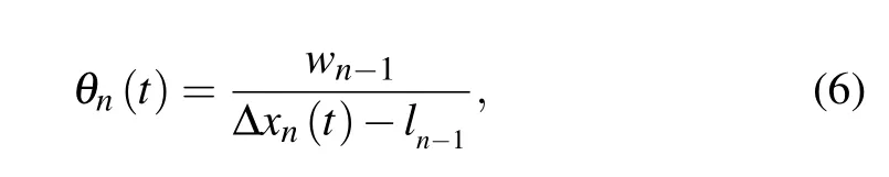
whereθn(t)is defined as the visual angle which is measured by the driver of thenth car at timet，Δxn(t)=xn+1(t)-xn(t)is the headway between the preceding (n+1)th car and the followingnth car，andln-1andwn-1represent the length and the width of the(n-1)th car，respectively.

Fig.1. Car-following model considering the visual angle.

In view of the above knowledge， we developed an improved car-following model considering the visual angle and anticipated time with stabilizing driving behavior.The dynamical equation is proposed as follows:

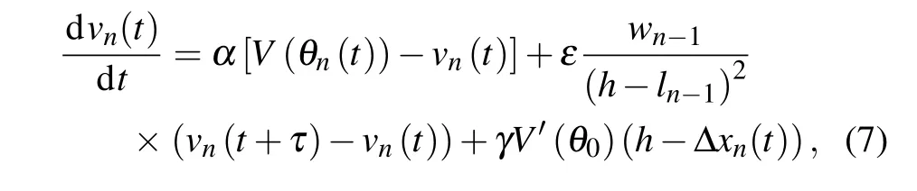
whereαis known as the sensitivity coefficient of drivers to the difference between the current speed and desired speed.vn(t)denotes the speed of carnat timet，εandγare defined as the sensitivity parameter of time-delayed velocity difference and steady-state control effects respectively， andτis the anticipated time. Furthermore，Vrepresents the optimal velocity whose mathematical expression is defined as follows:

whereve=maxV(x)＞0 is called the desired speed.

Equation (7) proved that the visual angle stimulus can really affect the response of driver to follower. Since carfollowing behavior is closely related to human decisionmaking and response，it needs to take human’s limits on judging headway and velocity stimulus into account. Therefore，considering driver’s visual angle factor can fit to the real traffic flow better.

3. Linear stability analysis

In this section， we conduct the prerequisites for the stability of the improved model by linear analysis. For a uniform traffic flow，all vehicles have the same characteristics，including everyone in the unified system is moving at the optimal velocityV(θ0)and the same headwayh，and the visual angleθn(t)remains the same. Obviously，we can obtain

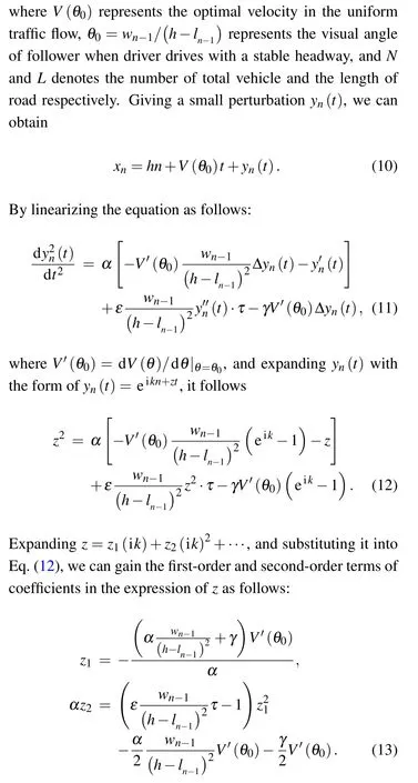
Integrating the two formulas， we can obtain the neutral stability conditions

With small disturbances，the neutral stability condition of the uniform traffic flow is as follows:

Whenαis satisfied with the condition， the traffic is stable with small disturbances.Otherwise，the traffic will become unstable.

Fig.2. Neutral stability curve with different γ，w，ε and τ.

Figure 2 depicts the neutral stability curve which describes the functional relationship between the headway and sensitivity coefficient space. As we can see，every neutral stability curve has a critical point (hc，αc) with differentγ，w，εandτ， respectively. The stability graph is separated into two parts by the critical curve， among which， one represents stability region，and the other represents instability region. Each point on the line represents a critical point for the stability to instability region. Whenα ＞αc， regardless of the headway，traffic flow will always remain stable， otherwise congestion may occur. In other words， the traffic flow will keep going above the neutral stability curve and congestion is impossible to happen. While under the curve，the traffic flow density increased along with the increased possibility of congestion.As shown in Figs. 2(a)， 2(c) and 2(d)， when fixing other parameters at a proper value，the vertices of the curve gradually decrease with the increases ofγ，εandτrespectively. However，they play different roles for traffic flow stability. Instead，Fig.2(b)describes the instability regions increase with the increasing ofwgradually when fixingε=0.2 s-1，γ=0.2 m-1andτ=0.5 s. From this， we conclude thatγ，εandτhave a positive effect in the traffic stability，which is opposite tow.

4. Bifurcation analysis and simulation

In this section，we use the theoretical analysis to explore the bifurcation behavior of the new model first of all so as to study the correspondence between the critical point of Hopf bifurcation and instability， and then conduct the numerical simulation to display the impact of various parameters on the bifurcation behavior intuitively. Equation(7)can be rewritten as

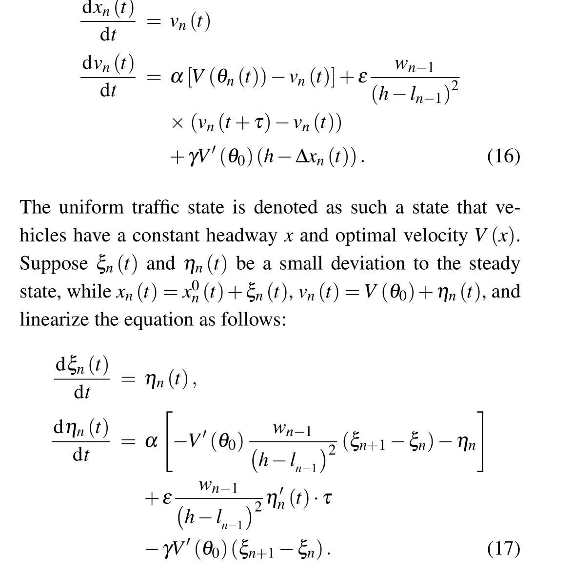
Through analyzing Eq.(17)，we obtain the linearized equation as follows:

Use the Hopf theorem to find the Hopf bifurcation pointL*.It can be found that when a smooth family of eigenvaluesλ=ψ±iωappears， the Hopf bifurcation condition is satisfied，and the bifurcation occurs.

Substitutingλ=ψ±iωinto Eq.(19)，one obtains

wherek ∈{1，2，...，N}.

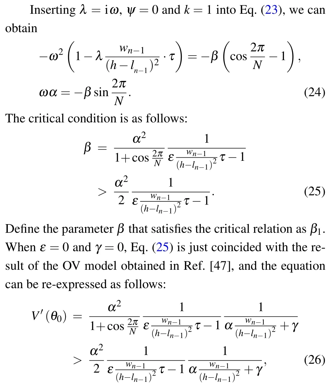
Separating the real and imaginary parts of Eq. (22)， the result shows

When Hopf bifurcation happens， there are only a pair of imaginary rootsλ1，2=±iω. In Fig. 3， all of other (N-2)eigenvalues are located in the left complex plane when a pair of pure imaginary roots appears at the first time(fork=1 andk=N-1).

Fig.3. Eigenvalues of the system for N=5，α =1 s-1，ε =0.05 s-1，and τ =0.4 s.

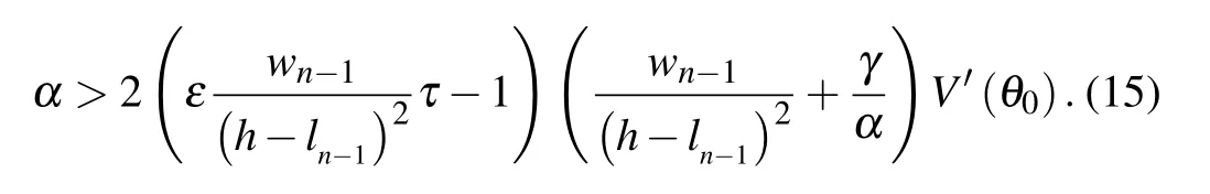
which is just contrary to the result shown in Eq.(15).

Next， differentiation of the characteristic Eq.(27)brings about the essential condition for the Hopf bifurcation，i.e.，

Obviously， from Eq. (27)， the Hopf conditionψ(β1)＜0 is satisfied absolutely. Therefore，the Hopf bifurcation occurs in our system. We can obtain the critical lengthL*from the following equation:

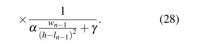
The spatial variation of Hopf’s relation(28)is displayed in the three-dimensional diagram of Fig. 4. The yellow surface is graph of

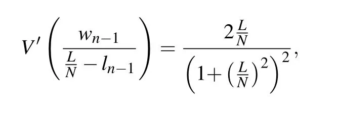
while the blue surface is the spatial variation curve of

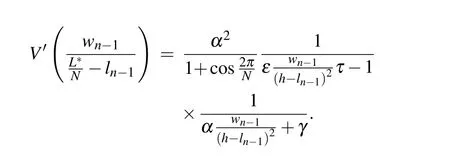
The intersection of these two surfaces corresponds to the critical point when Hopf bifurcation occurs.

In order to display and compare the effect ofτ，εandγon Hopf bifurcation more intuitively， Fig. 5 shows the two-dimensional(L，N)-plane corresponding to Fig.4，respectively，which reveals the instability regions of the system，and in which the first pair of eigenvalues have positive real parts drawn in yellow. The Hopf curve consists of the set of all intersections(L，N)of the first pair of eigenvalues and the second pair of eigenvalues， that is， the boundary between the blue plane and the yellow plane in Fig. 4. It is uncovered that the sensitivity anticipated timeτ，εandγplay a different role on the occurrence of Hopf bifurcation. Figures 5(a) and 5(b) indicate the critical point (LC，NC) of Hopf bifurcation from(4.1，3.8)to(5.1，8.9)because of the increasing of anticipated timeτfrom 1 to 2 and fixing the sensitivity coefficientε=0.05 s-1andγ=0.8 m-1.In Figs.5(c)and(d)，the critical point(LC，NC)of Hopf bifurcation changes from(4.1，3.8)to(5.4，10.8)with the increasing ofεwhile keeping anticipated timeτandγunchanged. It displays the instability area decreases because of the increasing ofε. In Figs.5(e)and 5(f)，the critical point (LC，NC) of Hopf bifurcation changes from(5.8，11.6) to (3.9，1.8) with the decrease of the sensitivityγand fixing the anticipated timeτ=0.4 s andε=0.05 s-1.It shows the instability area increases with the decrease ofγfrom 0.8 m-1to 0.65 m-1. Therefore， parameterτ，εandγall can inhibit the occurrence of bifurcation，it means they all contribute to the system’s stability despite the different effect in the critical point region of Hopf bifurcation.

Fig.5. Side view for α=1 s-1，ve=1 m/s with different values γ，ε and τ: (a)τ=1 s，ε=0.05 s-1，γ=0.8 m-1;(b)τ=2 s，ε=0.05 s-1，γ =0.8 m-1; (c) τ =1 s， ε =0.05 s-1， γ =0.8 m-1; (d) τ =1 s， ε =0.1 s-1， γ =0.8 m-1; (e) τ =0.4 s， ε =0.05 s-1， γ =0.8 m-1; (f)τ =0.4 s，ε =0.05 s-1，γ =0.65 m-1.

5. The TDGL eqnarray

In this section， we carry out the nonlinear analysis of Eq. (7) so as to obtain the TDGL equation that fits the improved model traffic behavior best near the critical point(hc，αc). The slow scales for space variablen， time variabletand constantbare introduced，and the slow variablesXandTare defined as follows:

While Δxn(t)is defined as follows:

wherehcstands for safety distance. By inserting Eqs.(29)and(30)to Eq.(31)，along with the Taylor expanding to the fifthorder ofμ，the nonlinear partial differential equation is shown as follows:

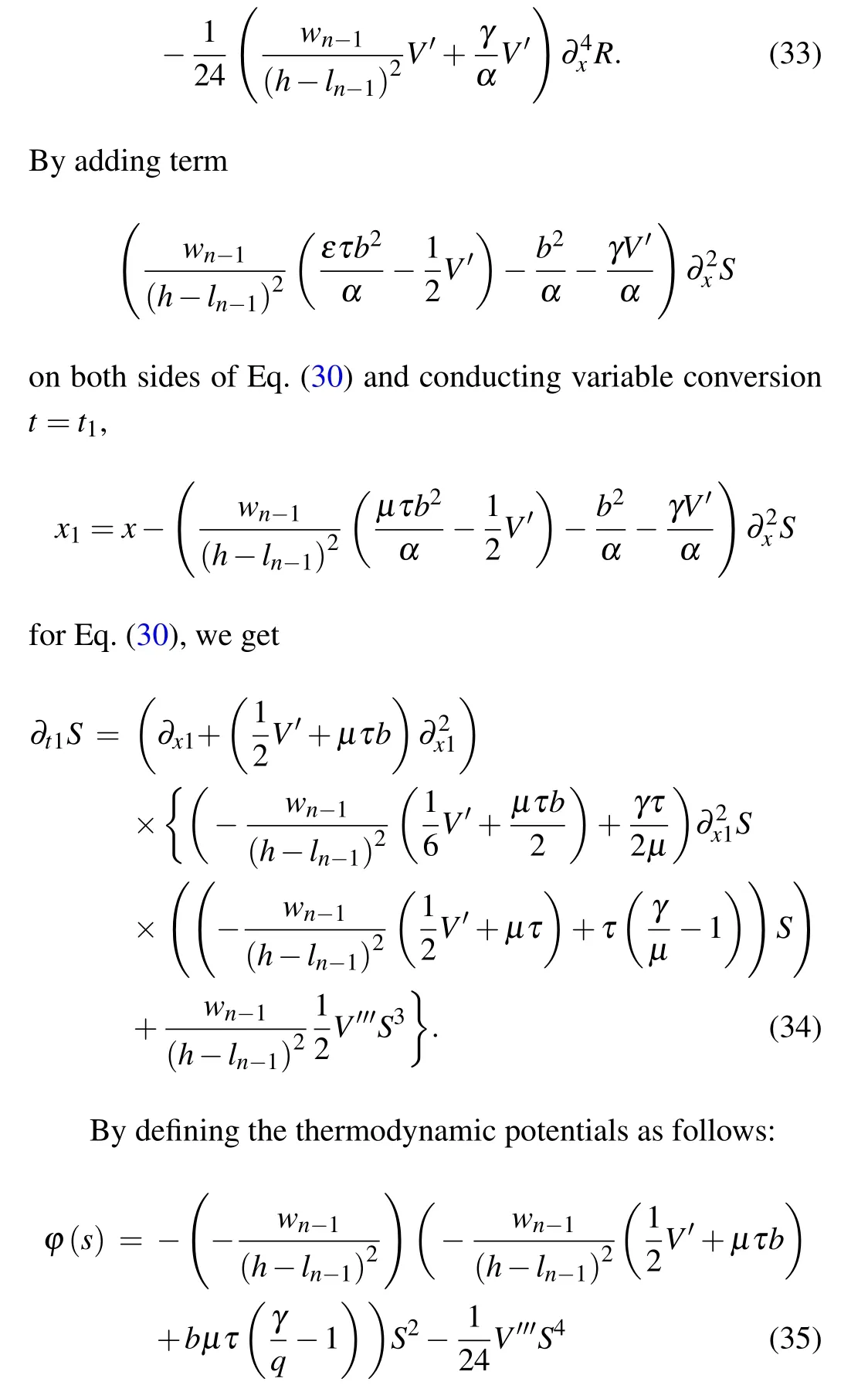
and substitute Eq. (35) into Eq. (34)， the TDGL equation is transformed as

where∂Φ(S)/∂Srepresents the function derivative. In addition to the simplest solutionS=0，another two stable solutions have also been shown，one of which is a uniform solution

and the other is the kink solution

wherex0is constant. Through analyzing Eq.(39)，we can obtain a coexistence curve when following formula relations are met:

Inserting Eq.(35)into Eq.(40)，we can obtain the coexistence curve with the original parameters

The spinodal line is based on the following conditions:

By inserting Eq.(35)into Eq.(42)，the relationship of the spinodal line is as follows:

Based on the condition∂φ/∂S=0 and Eq.(43)，we can calculate the critical point containing the original parameters

6. The mKdV equation

All ofgiare shown in Table 1.

Table 1. The coefficients gi.

In the table

In order to export the regularized equation，we give the following definition:

So，the standard mKdV equation withO(μ)correction term is obtained as

Then，assuming thatR′(X，T′)=R′0(X，T′)+μR′1(X，T′)and considering theO(μ) correction term， in order to obtain the propagation velocitycfor the kink solution，it can be based on the solvability condition as

where

and the general velocitycobtained by calculation is as follows:

whereV′′′＜0， andτrepresents the reciprocal of the driver’s sensitivity coefficient.

7. Simulation

7.1. Parameter calibration

In this part， 558 groups datasets of the 59th vehicle in the NGSIM database including velocity，acceleration and other factors are used to calibrate the optimal parameters. Considering that the modified dataset includes vehicle data in a noncar-following state， and existing the lane-changing behavior，therefore we make the following restrictions on car-following behavior.

(1)Car-following behavior should occur in the same lane，in other words， the data bar of Lane-ID should be the same value.

(2) Except for the first car， the selected leading car and following car，namely，preceding and following are not 0.

(3) In order to ensure that the vehicle stays in the carfollowing state， the headway should not be too large. Otherwise，the behavior change of the previous car will hardly affect the behavior of the target car.

Filtering by the above conditions，we can obtain the carfollowing data about the 59th car. Following is a partial data display.

Table 2. Car-following partial data of the 59th car.

According to the model in this article，we can determine the parameters to be calibrated in this article and the input variables of the car-following model， then using the least square method to perform nonlinear optimization of the calibration parameters. The specific objective function expression we adopt is proposed by Ossenet al.，[37]whose core idea is as follows:

whereNis the data group number，jdonates the serial number of data，andrepresent actual acceleration and simulated acceleration respectively. Meanwhile， as an evaluation index describing the fitness of the parameter calibration， the smaller the PI， the closer the measured value is to the simulated value， that is， the better the applicability of the fitting result.

Moreover， both models select parameter combinations optimized by genetic algorithm and within 5% of the error range as their analysis objects.Then normalize each parameter and systematically cluster the optimized processing results of each parameter，the comparison of each parameter distribution of the clustering results of the two methods in Table 3.

As we can see in Table 3 that considering the anticipated time and stabilizing driving behavior can decrease the influence ofαwith the same data， which means anticipated time and stabilizing driving behavior can eliminate or weaken the adverse effects of optimal velocity in unified traffic flow effectively. In addition， the smallerhand the increase ofvmaxindicate that the minimum safety headway requirement is smaller in the stable traffic flow，and the maximum velocity that each vehicle can reach in the traffic flow has increased，which means the extended VAM is easier to steady than the VAM.

Table 3. Calibrated parameters.

Figure 6 displays the fitness between the simulations and observations. It is not difficult to see that the red and pink curve maintain roughly the same trend with the blue line，where the pink and red lines denote the fitted value of extended VAM and VAM respectively， and the blue line represents the actual observation， indicating that the initial calibration coefficient set of the VAM and the extended VAM both can effectively predict the movement trend of the actual traffic flow during the acceleration，uniform velocity and deceleration phases.However，comparing the red and pink lines，obviously，the fitted value set of the extended VAM is closer to the observation in most data despite larger deviations in a few inflection points. And synthesizing the error value of all the data， it is found that the PI value is reduced from 0.6624 to 0.6237 after considering the gain and time-delay feedback control， which means that the controlled visual angle model can better reflect the complex actual flow.

7.2. Numerical simulation

In this section， numerical simulation of the improved model has been conducted so as to prove the obtained conclusions by using discrete equations. The discrete process is as follows:

In Fig. 7， the improved car-following model carries out a series of simulations while controlling other parameters unchanged. The patterns in Figs. 7(a)–7(d) correspond to the variablew(w= 1.6，1.8，2.0，2.2) respectively. Especially，whenw=1.6 m，the traffic flow has the highest stability that means the car width of the front car has a certain influence on the follower’s visual angle. As we can see that giving a small perturbation can induce initial stable traffic flow into an oscillating density wave. It can be clearly seen from the curvature change in Fig. 7 that the amplitude of the kink–antikink solution gradually increases with the increasing of parameterw.In other words，taking the vehicle width of the leader into account will interfere with the follower’s perspective，which will inevitably affect the stability of the system and increase the possibility of congestion at the same time. The wider the vehicle’s width，the more it can interfere with the driver’s perspective， and the greater the possibility of the system’s transition to instability region and traffic jams.

Figure 8 displays that the headway profiles and density waves for the preceding vehicle widthwatt=6000 s corresponding to panels in Fig. 7 respectively. Obviously， as the width of the vehicle increases， the amplitude of the headway gradually increases，which means considering the width of the leader will restrain the stability of the traffic flow and prolong the time for the unstable traffic flow to stabilize.

Fig.7. Space–time evolution of the headway from with the t=5000 s to 6000 s.

Fig.8. Headway profiles of the density wave at t=6000 s correspond to Fig.6 respectively.

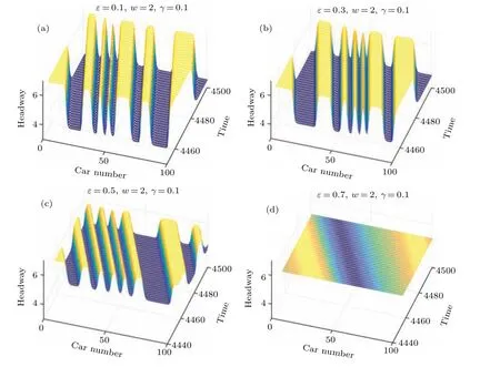
Fig.9. Space–time evolution of the headway from with the t=4400 s to 4500 s.

In Fig.9，we explore the effect of the anticipated time on the stability of traffic flow in the improved car following model through a series of simulations， where Figs. 9(a)–9(d) correspond toε(ε=0.1，0.3，0.5，0.7)，respectively. It can be obviously seen from the change curvature in Fig.8 that considering the anticipated time contributes to stable movement of the system. Specially，whenε=0.7 s-1，the density wave change curvature is zero， at this time， the traffic flow steadily travels with a constant headway，and the entire traffic flow system has the highest stability. Therefore，we conclude that considering the driving characteristics of subject driver can effectively improve the stability of the traffic flow. The proposed new model considers the anticipated time and the subject driver uses the received original traffic information combines with his own prediction of the front traffic state to shorten the time responds to the front traffic situation， which provides a comprehensive improvement to the entire car-following behavior.

Figure 10 displays the headway profiles and density waves for anticipated time att=4500 s corresponding to panels in Fig. 8 respectively. From Figs. 10(a)–10(d)， considering the speed difference，the traffic congestion conditions can be effectively alleviated，and as the anticipated time increases，the amplitude of the density wave gradually decreases，which means the traffic flow tends to move with a stable headway.The improved model has improved to a greater extent in eliminating interference. From Fig.10，we obtain that parameterεcan promote the stability of traffic flow.

Fig.10. Headway profiles of the density wave at t=4500 s correspond to Fig.8 respectively.

Figure 11 mainly depicts the hysteresis loop relationships between the velocity and density， which are shown with deferentγ(γ=0.05， 0.1， 0.15， 0.2)respectively. As we can see the size of the loop gradually decrease with the value increasesγin Fig. 11. This also means that considering driver’s stabilizing driving behavior can effectively ease traffic congestion and promote the stability of the system at the same time.

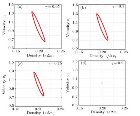
Fig. 11. The hysteresis loops relations of the velocities v1(t) and the density ρ1(t)=1/Δx1(t)respectively.

8. Conclusion

In this paper， we take the anticipated time and stabilizing driving behavior into the visual angle model， combining anticipated time with stabilizing driving behavior to explore driver’s sensitivity of change of angle information. The relationship of neutral stability is obtained by linear stability analysis. Meanwhile， bifurcation analysis for the improved carfollowing model considering the visual angle，anticipated time and stabilizing driving behavior is investigated. Hopf bifurcation analysis mainly consists of two modules， one is theoretical analysis and the other is numerical simulation. Through the Hopf bifurcation analysis we can obtain the critical points.Results show that bifurcation analysis results are highly coincide with the stability condition of linear stability analysis.Furthermore，from the three-dimensional bifurcation diagram，it is found that the critical points of Hopf bifurcation are located on the boundary between the stability region and the instability region. Hopf bifurcation leads to conversion of stable traffic flow to irregular traffic flow. In addition， the TDGL equation is obtained by nonlinear analysis，and then the coexistence curve，metastable curve and critical point are described according to the obtained thermodynamic potential.We obtain the mKdV equation of the model in the same way. Finally，the parameter calibration and numerical simulation results display that the anticipated time and stabilizing driving behavior both play a positive role on traffic flow， which is opposite to the visual angle. Based on the conclusions， the article will make contributions on providing theoretical support for the establishment of intelligent transportation systems and references for traffic management systems.

Acknowledgements

Project supported by the Natural Science Foundation of Zhejiang Province， China (Grant Nos. LY22G010001，LY20G010004)， the Program of Humanities and Social Science of Education Ministry of China (Grant No. 20YJA630008)， the National Key Research and Development Program of China-Traffic Modeling， Surveillance and Control with Connected & Automated Vehicles (Grant No. 2017YFE9134700)， and the K.C. Wong Magna Fund in Ningbo University，China.