Yaxian MA (麻雅娴)

School of Science，North University of China，Taiyuan 030051，China E-mail:myxyxx1994@163.com

Xianwen ZHANG (张显文)†

School of Mathematics and Statistics，Huazhong University of Science and Technology，Wuhan 430074，China E-mail:xwzhang@hust.edu.cn

Abstract We consider asymptotic behaviors of the Vlasov-Poisson system with radiation damping in three space dimensions.For any smooth solution with compact support，we prove a sub-linear growth estimate of its velocity support.As a consequence，we derive some new estimates of the charge densities and the electrostatic field in this situation.

Key words Vlasov-Poisson system;radiation damping;asymptotic behavior;velocity support

1 Introduction

This paper is concerned with the asymptotic behavior of the classical solutions to the three dimensional Vlasov-Poisson system with radiation damping.The system has been established by Kunze and Rendall[11，12]and reads as follows:

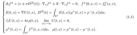
Here f+(t，x，v) and f-(t，x，v) are the phase-space densities of positive and negative particles，respectively，at time t≥0 and position x∈R3，moving with velocity v∈R3，and where ρ(t，x)，U (t，x)，E (t，x) and σD[2](t) are the net charge density，the potential，the electrostatic field and the radiation damping of the system，respectively，with σ∈(0，1]being a small constant characterizing the magnitude of the radiation damping.Note that for the sake of simplicity，the mass and the charge of the two kind of particles have been normalized to 1 and±1，respectively.In what follows，we assume that the initial dataare given nonnegative functions verifying

If we ignore the radiation damping (namely σ=0) and consider a monopolar particle system (say e.g.:f-≡0)，then (1.1) degenerates to a special case of the classical monopolar Vlasov-Poisson system:

Here E (t，x) represents a gravitational field when γ=-1 and a repulsive field when γ=1.The system (1.3) has been extensively studied in recent decades (see，e.g.:[7，22]and the references therein).Specifically，the global existence of classical solutions for general data was independently established in two different ways:the Euler approach[13]and the Lagrange approach[20].Based upon the first method，the propagation of velocity moments or velocityspatial moments have been thoroughly studied (see，e.g.:[1，5，6，17-19]).On the other hand，the asymptotic behavior of the system in terms of estimating the largest velocity R (t)=sup{|v|:(x，v)∈suppf (t)}has also received a great deal of attention in the framework of the Lagrange approach[3，4，9，10，14-16，20，21，23].

As for the Vlasov-Poissonsystem with radiation damping (1.1)，the global existence，uniqueness and decay estimates of classical solutions with compact support were established in[12]by the Euler approach，and propagation for any velocity and velocity-spatial moments of order＞2 was investigated in[26].The existence and uniqueness of global-in-time solutions with finite or in finite energy were proved in[2，25].However，until now，there has been no research on the asymptotic estimate of the largest velocities.The purpose of this paper is to analyze rigorously the asymptotic growth bounds for the velocity support of the system (1.1).The main result can be stated as follows:

Theorem 1.1Let initial datasatisfy (1.2) and let f±(t，x，v) be a classical solution to system (1.1).Then there exists a constant C＞0 such that，for all t≥0，

where

P±(t)=sup{|v|:(x，v)∈suppf±(s)，s∈[0，t]}.

Consequently，the charge density and the field E (t，x) have the following estimates:

‖ρ±(t)‖∞≤C (1+t)67/28，‖E (t)‖∞≤C (1+t)46/63，∀t≥0.

System (1.1) will degenerate to the three dimensional bipolar Vlasov-Poisson system when σ=0.For the later system，under the assumption of electric neutrality，some better results have already been obtained for dimensions one and two (see，e.g.:[8，24]).In this paper，for a set Ω，1Ωdenotes its indicator function，the Lpnorm is denoted by‖·‖p，and C denotes positive constants changing from line to line and depending only on.In addition，∨and∧are logical symbols referring to“or”and“and”，respectively.

2 Preliminaries

In this section，we collect some important conclusions and a priori estimates obtained in[12].The first one is about the existence of a global classical solution.

Proposition 2.1Ifsatisfy (1.2)，then there exists a unique solution f±(t，x，v)∈C1([0，∞]×R3×R3) to the system (1.1).

Letting f±(t，x，v) be the solution to system (1.1) given by Proposition 2.1，the characteristic system

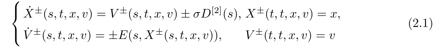
has a unique C1solution (X±(s，t，x，v)，V±(s，t，x，v)).

Lemma 2.2Letting (X±(s，t，x，v)，V±(s，t，x，v)) be the characteristic flow given above，the solution to system (1.1) can be expressed as

As a consequence，we have that

The mapping (x，v)∈R3×R3(X±，V±)(s，t，x，v)∈R3×R3is C1homeomorphic and measure preserving for all fixed s，t∈[0，∞).Moreover，for all t≥0，we have that

Then we turn to the decay estimates for quantities related to the system.The kinetic and potential energies are defined by

and

so the total energy is computed by

E (t)=Ekin(t)+Epot(t).

Lemma 2.3The solution f±(t，x，v) defined in Proposition 2.1 satisfies

Furthermore，it holds for all t≥0 that

where C and C*are constants depending only on.

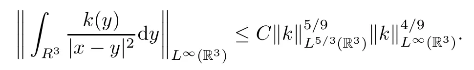
Finally，we recall the following standard lemma (see e.g.:[15]):

Lemma 2.4Let k∈L∞(R3)∩L5/3(R3).Then，

3 Proof of Theorem 1.1

To establish the estimate (1.4)，we denote for Δ∈[0，t]that

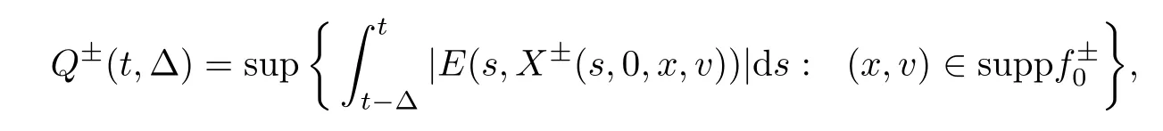
and

Q (t，Δ)=Q+(t，Δ)+Q-(t，Δ).

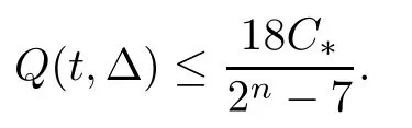
Then，for any fixed t≥0 and n≥3，let

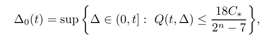
where C*is the constant in (2.5).If Δ0(t)=t，then for all Δ∈(0，t]，

According to the characteristic system (2.1)，we know that

As a consequence，by Lemma 2.2，we have that

P±(t)≤r0+Q±(t，t)≤C，

and the estimate (1.4) is obvious.

If Δ0(t)＜t，we have Q (t，Δ0(t))=and Q (t，Δ)≤for all Δ∈[0，Δ0(t)]，because Q (t，Δ) is a nondecreasing function with respect to Δ∈[0，t].On the other hand，for Δ∈[Δ0(t)，t]，we need to handle it with great care.

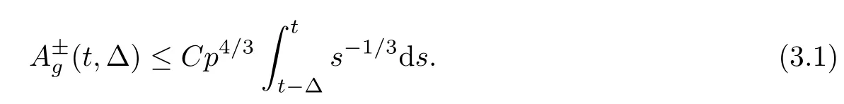
Proposition 3.1Let the nonnegative datasatisfy (1.2).For any fixed t≥r0，if Δ0(t)＜t，then there exists a constant C＞0 depending onsuch that，for all Δ∈[Δ0(t)，t]and t-Δ≥1，

where ln+denotes the positive part of ln，p=2n+1Q (t，Δ) and r＞0.

ProofFor the sake of simplicity，we denote

For the sake of simplicity，we denote

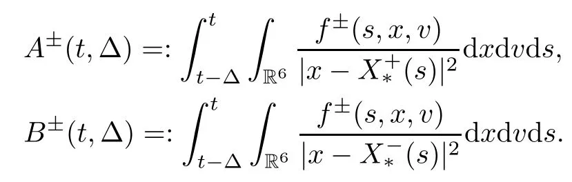
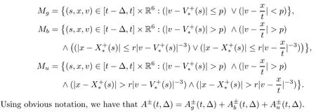
The estimate of B±(t，Δ) is similar to that of A±(t，Δ)，so we just need to investigate A±(t，Δ).For parameters p＞0 and r＞0，which are to be specified later，we split the domain of integration in the A±(t，Δ) as follows:

The contribution ofMg.We have that

Now，in consideration of Lemma 2.4，we obtain

and conclude that

The contribution ofMb.We have that

We estimate I1and I2separately.Due to Lemma 2.2，|v|≤P (s)≤P (t) and|v-|≤2P (s)≤2P (t) for v∈suppf±(s，x，·)，s∈[t-Δ，t].Thus，by (2.2) in Lemma 2.2，we have that

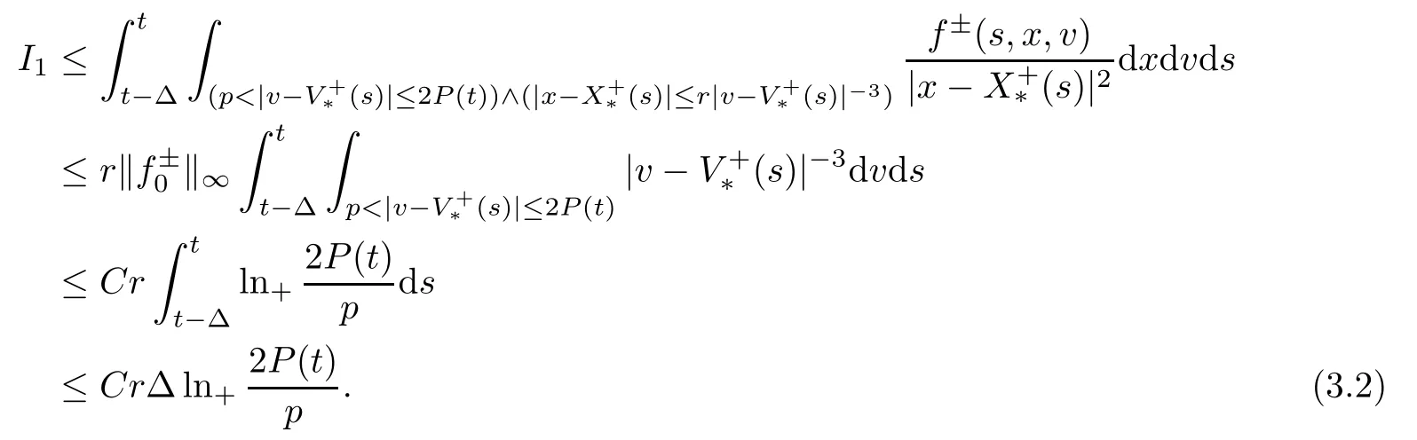
If p is bigger than 2P (t)，the corresponding integral is zero.As for the second term I2，using (2.5) in Lemma 2.3 and t≥r0，we note that

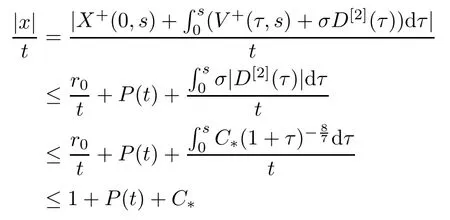
for s∈[t-Δ，t]and (x，v)∈suppf+(s).Similarly to I1，we have≤1+2P (t)+C*and

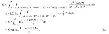
Combining (3.2) with (3.3)，we obtain

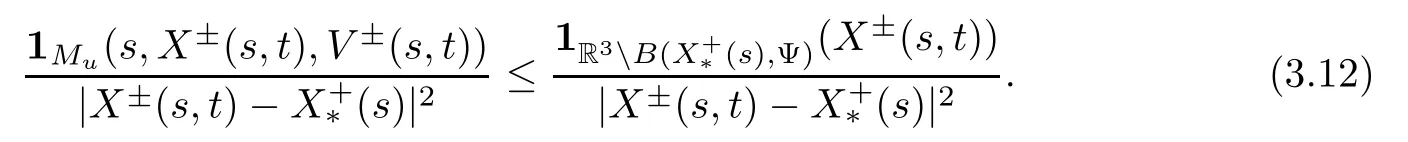
The contribution of MuThe main idea in estimating the contribution of the set Muis to integrate with respect to time first.By a changing of variables (x，v)→(X±(s，t)，V±(s，t))，we have that

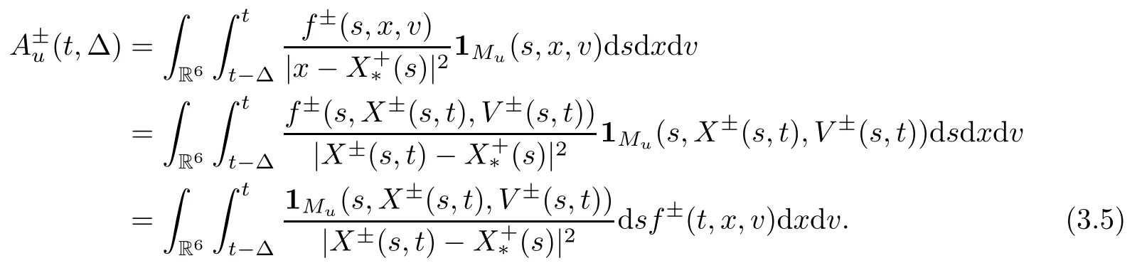
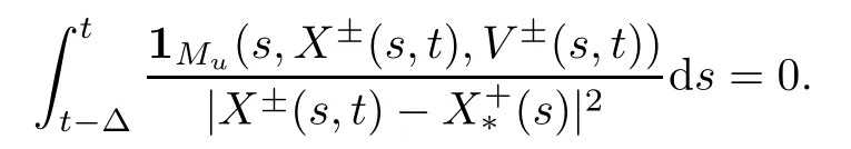
Now we consider the integral with respect to s.If (s，X±(s，t)，V±(s，t))Mufor s∈[t-Δ，t]，then

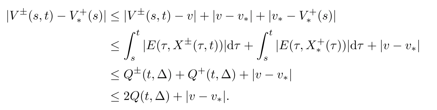
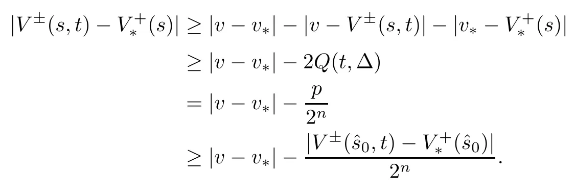
Together with the definition of Q (t，Δ) and the triangle inequality，we have for s∈[t-Δ，t]and (x，v)∈suppf±(t) that

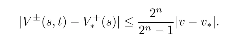
By the choice of p and (3.6)，we have that

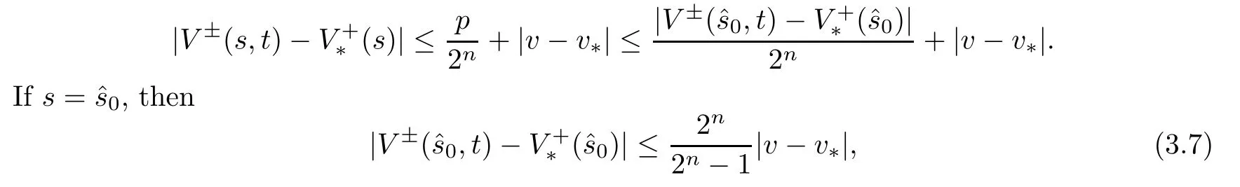
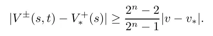
which implies that

Similarly，

According to (3.7)，we get

Consequently，we obtain，for all s∈[t-Δ，t]，that

Due to t≥1，from

and the choice of p，we obtain

Then，applying (3.6)，we have that

Substituting this estimate into (3.9)，we get

Therefore，by (3.8)，(3.10) and n≥3，we obtain

for all (s，X±(s，t)，V±(s，t))∈Mu.We denote

Consequently，

Define

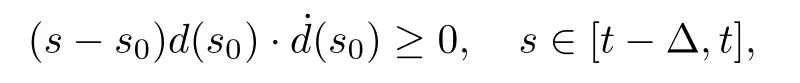
We Taylor-expand this difference to first order around a point s0∈[t-Δ，t]which is defined by

We have

According to the definition of Q (t，Δ) and (2.5)，we obtain

By the definition of s0in (3.13)，distinguishing the cases s0=t-Δ，s0∈(t-Δ，t) and s0=t，we see that

and thus，

Applying (3.8)，we have

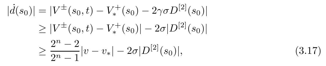
so we conclude，from (3.14)-(3.17)，that

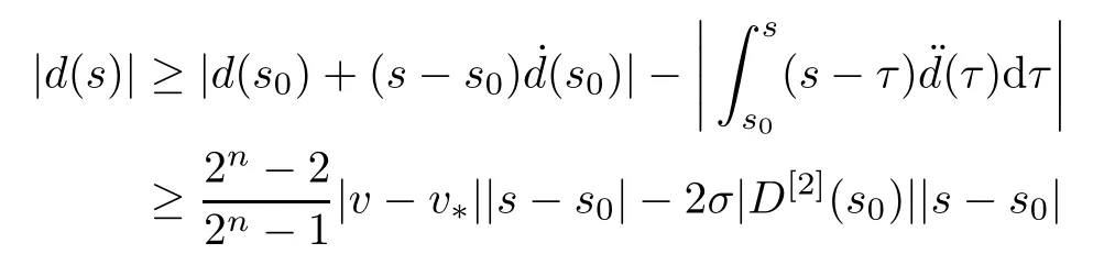
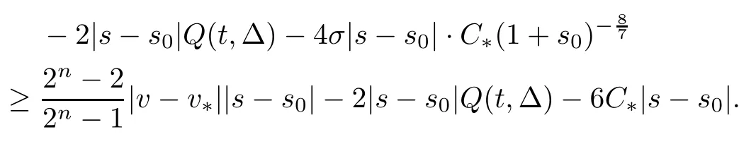
Combining the choice of p and (3.7)，we know that

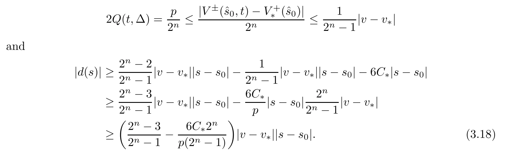
In particular，from Q (t，Δ0(t))=and the assumption of the proposition，we know that

Inserting this into (3.18)，we get

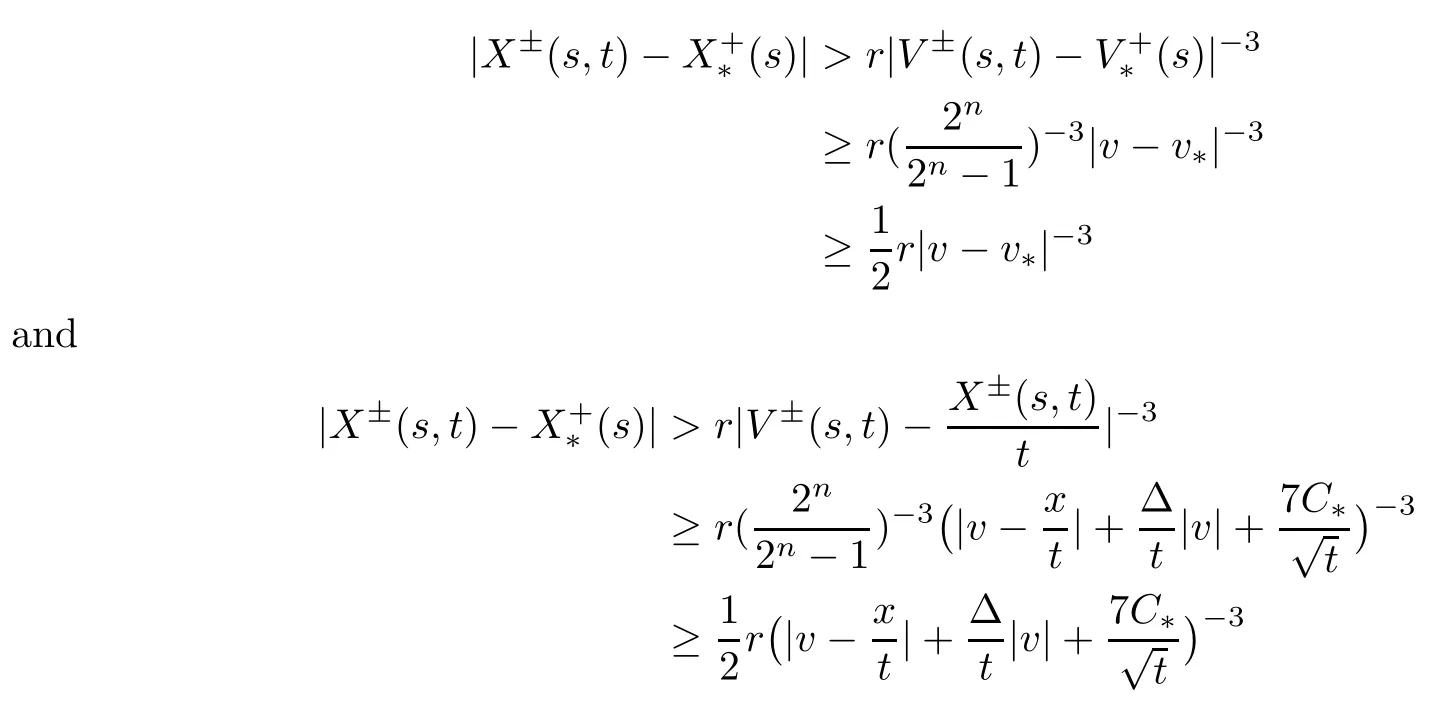
It is now time to estimate the integral with respect to s on (3.12).We define auxiliary functions

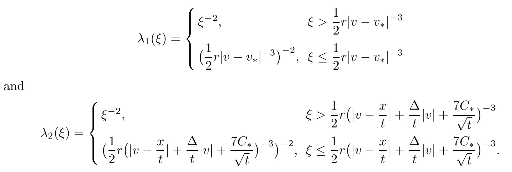
By (3.11)，(3.12)，(3.19) and the monotonicity of λi，we know that for i=1，2 and s∈[t-Δ，t]，

We can now estimate the time integral in the contribution of Muas follows:

Since this estimate holds for both i=1 and i=2，we have that

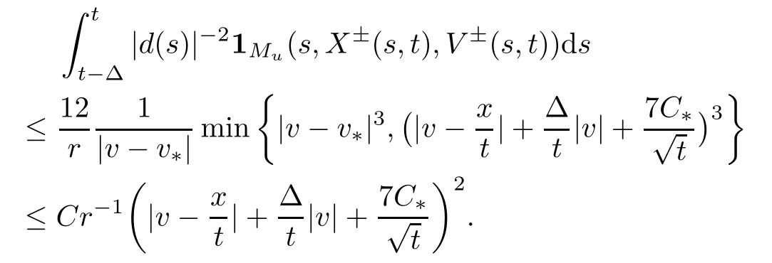
Combining this with (2.3) and inserting into (3.5)，we obtain

Combining the estimates (3.1)，(3.4)，and (3.20)，and observing the definition of Q+(t，Δ)，we get that

for all t and Δ such that t≥r0，Δ∈[Δ0(t)，t]and t-Δ≥1.Analogously，we can establish similar estimates for B±(t，Δ):

In the end，we obtain that

for all t and Δ such that t≥r0，Δ∈[Δ0(t)，t]and t-Δ≥1. □

Proof of Theorem 1.1In order to obtain an estimate for P (t)，we choose t*≥max{1，r0}such that

such t*exists，since

Now fixing t＞t*and letting n=log2(27C*t1/16+7)，we assume the first case，that is，

Denote

By (3.21) and (3.22)，we have that

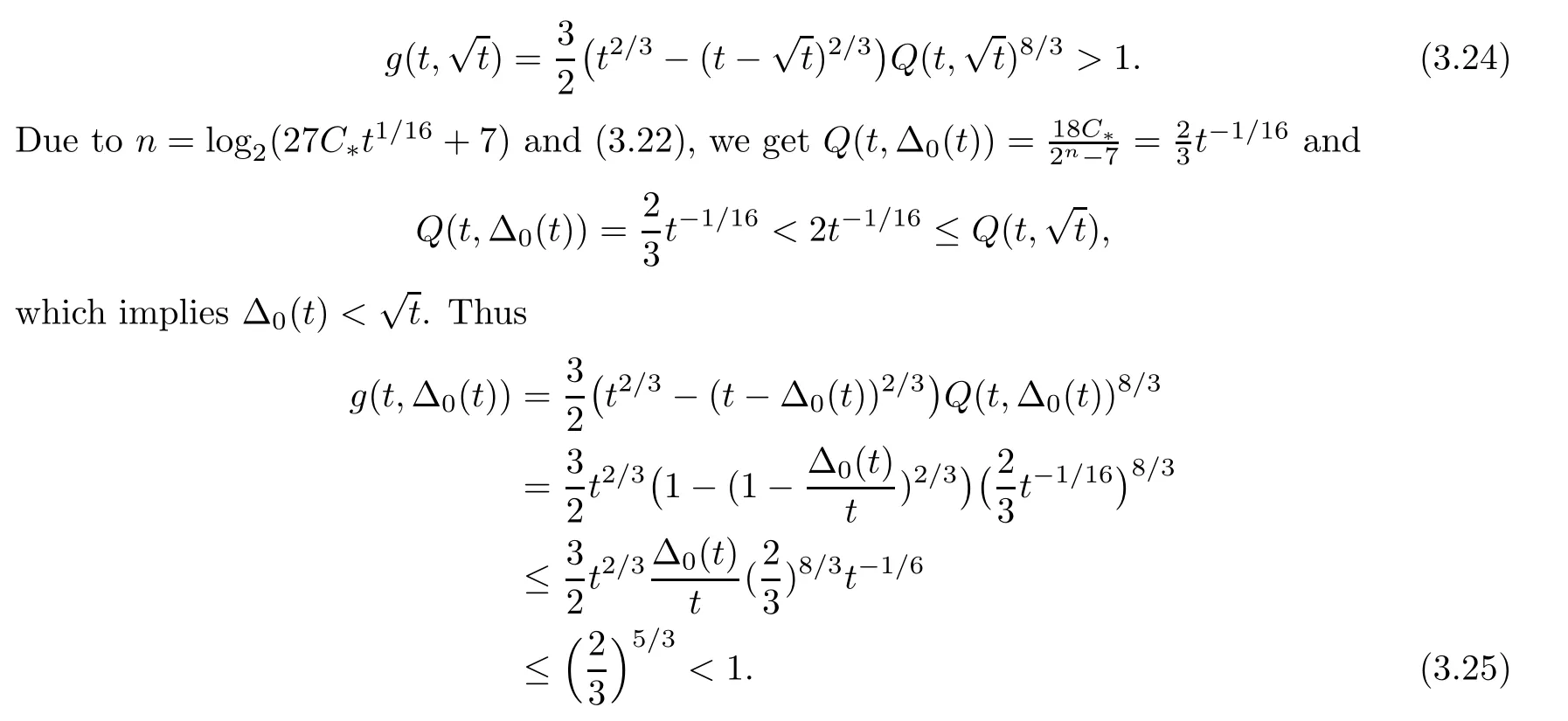
Since we have (3.24) and (3.25)，and g is a strict monotonicity continuous function of Δ，there exists a uniquesuch that

From the definition of g，we know that

Then we choose the parameter r as

Combining this with (3.27)，we obtain

and because we already have from[12]that P (t) is bounded by some power of t，we obtain the estimate

By (3.27) and (3.28)，we have that

In a word，when (3.22) is true for t≥t*，we can choose，and (3.29) holds true.In the other case，together with (3.21)，we have that

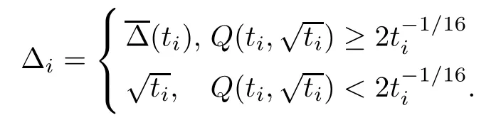
Next，let t1=t＞t*and ti+1=ti-Δi，as long as ti＞t*，where

Now，we prove that this process terminates after finitely many steps (i.e.，there exists k∈N such that tk-Δk≤t*＜tk).In the first case，we assume that the iteration is in finite，so→0.Because of (3.23) and the continuity of g，we know that g (limti，0)=0，which contradicts (3.26).Clearly，due to＞0，the other case happens only a finite number of times.Applying (3.29) and (3.30) repeatedly，we obtain

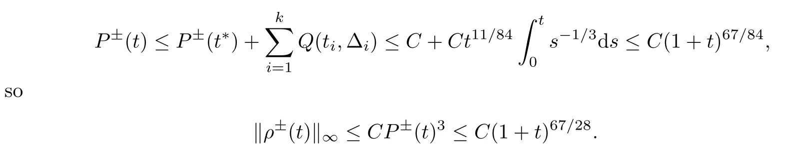
In addition，according to Lemma 2.4 and (2.4) in Lemma 2.3，we have that

and the proof is complete. □