Le Bai(柏乐) Ming-Lei Shan(单鸣雷) Yu Yang(杨雨) Na-Na Su(苏娜娜)Jia-Wen Qian(钱佳文) and Qing-Bang Han(韩庆邦)

1Jiangsu Key Laboratory of Power Transmission and Distribution Equipment Technology,Hohai University,Changzhou 213022,China

2College of Internet of Things Engineering,Hohai University,Changzhou 213022,China

Keywords: two-component lattice Boltzmann method,acoustic attenuation

1. Introduction

Acoustic attenuation is a process of estimating energy loss in sound due to its engendering through media,owing to mainly two mechanisms known as classical attenuation and relaxation attenuation.[1-5]Classical attenuation originates from transport phenomena of gases,which include viscosity,diffusion,and heat conduction.[6,7]In contrast,relaxation attenuation stems from thermal relaxation of internal degrees of freedom of polyatomic molecules.[8,9]The nonlinear relationship between relaxation attenuation and frequency makes it complex to understand attenuation effect of sound, which compels us to design an accurate acoustic attenuation prediction model.[10-12]

Energies are stored in the translational and inner degrees of freedom at equilibrium for gas at rest. If the gas is not at rest, external disturbances such as a passing sound wave may cause a change in its translational energy.This change will push the degrees of freedom into a out-ofequilibrium state, and a gradual readjustment to equilibrium will occur. This readjustment happens throughout molecular collisions.[13]The results predicted through the lattice Boltzmann model include classical attenuation, relaxation attenuation and attenuation caused by other effects, which can reasonably and accurately describe attenuation of sound waves in gases.

In recent years, the lattice Boltzmann method (LBM)has emerged as an effective computational method, which bridges the concept of micro-scale and macro-scale, known as the mesoscopic method.[14-19]Researchers previously used the single-relaxation-time(SRT)LBM model to simulate twocomponent mixtures.[20-26]Luoet al.established a unified approach for developing the lattice Boltzmann models to study the multi-component fluids within the kinetic theory framework.[27,28]Based on this theory,many efforts have been devoted to exploring the flow of binary mixtures.[29]At the same time, Zhanget al.extended the discrete unified gas kinetic scheme towards the study of flows in binary gas mixtures.[30]The self-collision term found in the abovementioned literature adopts the SRT or Bhatnagar-Gross-Krook (BGK) model. However, the numerical accuracy and stability of the BGK model are found to depend strongly on the relaxation time in the evolution equation.[31,32]The SRT model causes the numerical instability when the viscosity is too large or too small.

The process of LBM simulation of sound attenuation is closely related to various factors, predominantly viscosity,macroscopic velocity, and density. The LBM has been used as an extensive method to characterize the propagation properties of sound waves in gases.[33,34]Viscosity has a great influence on stability of the SRT model,[35-37]and the improved multiple-relaxation-time(MRT)model significantly improves the stability. The stability and accuracy of the calculation results of the MRT model under extreme viscosity, and the rationality of studying the LBM model through the sound attenuation model need to be resolved. Therefore, the present study presents a unique sound attenuation model to address the above-mentioned problems. The effect of the error term of the macroscopic equation on the calculation accuracy of the sound attenuation model is investigated and presented in Section 4.The results show that the error value of the sound attenuation coefficient can correctly reflect the error of the macro equation of the MRT-LBM model. It is perceived that the results of the MRT model stability and accuracy drawn by the sound attenuation model are general,which can be applied to different calculation models.

In this paper,an improved simulating model with an MRT collision operator is presented to study the flows of binary gas mixtures, and the equilibrium moment with the diffusion term is calculated. The rest of this paper is organized as follows. Section 2 presents an improved MRT-LBM model,and a detailed C-E expansion analysis is given in the appendix.In Section 3, the improved LBM model is used to simulate the diffusion phenomenon. Then the numerical stability and sound attenuation characteristics are also verified. In Section 4, the effects of viscosity, density ratio and concentration on the stability and accuracy of the MRT-LBM model are manifested. At the same time,the influence of the error term of the macroscopic equation on the calculation accuracy is analyzed.In Section 5, we draw summary of the current investigations along with the future research directions.

2. The two-component MRT-LBM model

Kinetic theory of gas mixtures has received much attention by the scientific community.[38,39]On the basis of kinetic theory, an SRT-LBE model with the BGK collision operator was proposed by Luoet al.[27]In order to improve the stability of the above model, we present an improved MRT-LBM model, and conduct a rigorous C-E expansion analysis. The evolution equation is expressed as

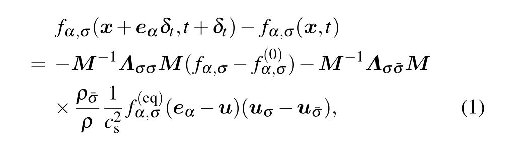
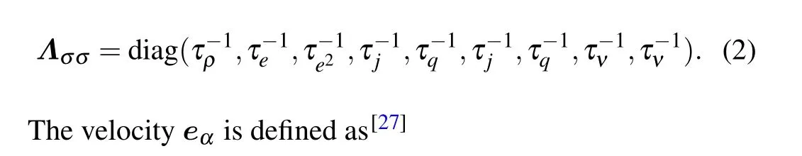
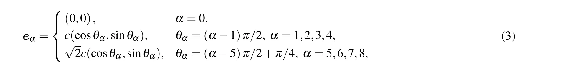
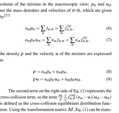
wherefα,σ(x,t) is the discrete density distribution function of componentσ,xis the particle position,δtis the time step,andαis the number of discrete velocities.In a binary mixture,σ=1,2, ¯σ/=σmeans different components.On the right side of the equation,the first term represents the self-collision term,and the second term represents the cross-collision term. For the D2Q9 lattice model,the orthogonal transformation matrixMis detailedly given in Ref.[40]. Here, the diagonal relaxation matrixΛσσis defined as[27]

This is the standard incompressible Navier-Stokes(N-S)equation. The C-E multi-scale analysis shows that the improved model can accurately restore the macroscopic mass and momentum conservation equations.

3. Verification of flow properties

In order to show whether the MRT model is proper for studying the flow of two-component mixtures, we simulated the phenomenon of binary diffusion. At the same time, the stability of the MRT model was tested with the SRT model.Then the sound attenuation prediction channel model was established to verify the accuracy of the model under different parameters.

3.1. Verification of diffusion phenomenon

Diffusion is the result of net movement of molecules driven by a gradient in the chemical potential of fluid species.[41-43]The advantage of the improved model is that it gives an equilibrium moment with a diffusion term, which makes the programming and calculation simpler. To verify the accuracy of the improved model,this section simulates the diffusion of binary mixtures. Notably,the diffusion process is found to be consistent with the physical phenomenon through the simulation process.

In Fig. 1, we show the initial configuration of the twocomponent diffusion. As is shown, there are two-component mixtures with different concentrationnσon the left and right sides of the container.

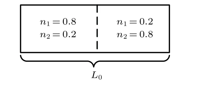
Fig.1. Initial configuration of the two-component diffusion.

The upper and lower boundaries adopt nonequilibrium extrapolation boundary conditions,and full developed boundary conditions are adopted in the left and right boundaries.The initial velocity of each component isuσ= 0, and the diagonal relaxation matrix isΛσσ= diag(1,Ωσ,Ωσ-1,1,1.2,1,1.2,Ωσ,Ωσ), whereΩσ=1/(3νσ+0.5),Λσ¯σ=Λ¯σσ=diag(1,2,2,1,1,1,1,2,2).

In fact,the diffusion phenomenon described in this article is a one-dimensional problem as the physical field is the same in the vertical direction.[32]In order to facilitate the setting of upper and lower boundary conditions, the mesh is chosen asNx×Ny=1000×3,the length of the channel model isL0,the spatial step isδx=δy=5/3×10-4l.u., and the time step is set asδt=5/3×10-4t.s. All units used in this paper are standard lattice units,t.s. means time step,m.u. and l.u. represent mass unit and lattice unit, respectively. The mole fraction is defined asXσ=nσ/n,wheren=n1+n2,and the range ofXσis 0-1.The analytical solution expression for the mole fraction of componentσis as follows:

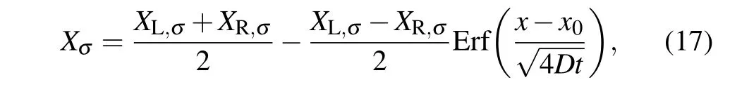
where Erf is the complementary error function,x0=L0/2 is the location of the interface,D=10-3is the diffusivity, and the subscriptsLandRindicate the left and right sides of the container.

As shown in Fig.2,the triangles and circles represent the simulation results of componentσ=1,2, respectively. Solid lines are used for the corresponding analytical solutions. Herexrepresents the distance from the left side of the container,the length of the channel model isL0, and the abscissax/L0represents the normalized distance.

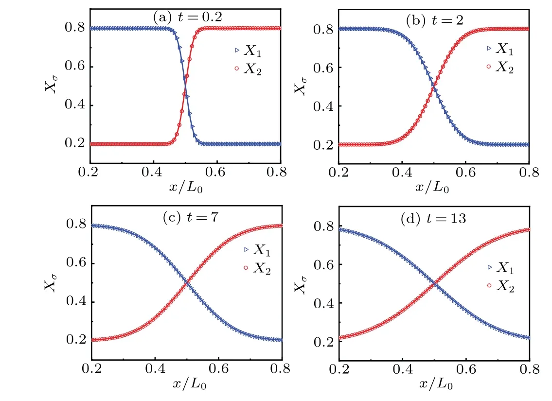
Fig.2. Molar fractions of the different component in the diffusion process.

Figure 2 shows the change of the mole fraction at different times during the diffusion process. The simulation results and analytical solutions at different timest=0.2,t=2,t=7 andt=13 time steps are found in good agreement. From this study, it is found that the presented MRT model can describe the flow between various components accurately.

3.2. Verification of numerical stability

It is known that the numerical stability of the lattice Boltzmann equation (LBE) is significantly influenced by the relaxation times, especially for shear viscosity.[21,26]The SRT model may lead to numerical instability if shear viscosity is too large or small. To check whether the presented MRT model can overcome these problems, we therefore analyzed the stability of the densitiesρσfor both the models of SRT and MRT.The range of shear viscosityνσis chosen from 0.001 to 1.5 l.u.2/t.s.,τσ=3νσ+0.5. When the density simulation result is stable, the error Δρσbetween the average value of the density at different positions and the theoretical value is calculated. The error expression is Δρσ=|¯ρσ-ρσ|, and the simulation results of the error Δρσare listed in Table 1.

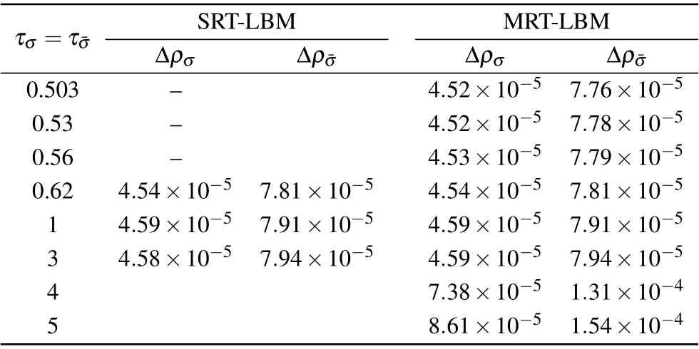
Table 1. Comparison of the equilibrium properties among the SRTLBM model and the present MRT-LBM model. The concentration ratio is 5:5 and the density ratio are ρ1:ρ2=1:2. The density error expression is Δρσ =|¯ρσ-ρσ|,where ¯ρσ is the average value of the simulated density of the horizontal centerline of the channel. The“-”sign represents the calculation result to be unstable.

The SRT model encounters numerical instability for small or large values ofτσ. Fortunately, the present MRT model works well noticeably for all cases.Henceforth,the simulation results confirm the superiority of the present models used in this study in terms of achieving the improved numerical stability. It is worth mentioning that the density stability decreases when the viscosity is high, which will reduce the calculation accuracy.

3.3. Verification of acoustic attenuation

Next, the MRT-LBM model has been implemented to simulate the sound attenuation in the binary gas mixture. In order to investigate the effect of viscosity, concentration, and density on the sound attenuation,the sound attenuation channel model has been designed in the following way as shown in Fig.3.

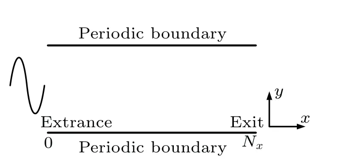
Fig.3. The sound attenuation channel model.

Sound waves propagate along thex-direction. The source of sound is located at the channel entrance,whose oscillation velocity is set tou0=uAsin(ωt), whereuAis the amplitude of the oscillation velocity andωis the angular frequency. The channel is filled with binary gas mixture. The boundary conditions are periodic in the vertical direction, an equilibrium boundary is adopted at the entrance,and the influence of sound reflection at the exit is not considered. A certain density disturbance is given at the sound source as follows:

whereρ0is the average of the theoretical values of the two component densities,δρis the density disturbance. Ifρ0=1 m.u./l.u.3andδρ=0.01 m.u./l.u.3, thenuA=csδρ/ρ0=0.00577 l.u./t.s. The mesh is chosen asNx×Ny=1000×3,the length of the channel model isL0, time step and spatial step are the same as those in the diffusion model. The analytical solution of this problem is given by the following equation:

Heretis the propagation time, and the sound attenuation coefficient isα=4π2ν0/csλ2, whereν0is the viscosity of the mixed components,and the expression isν0=(μ+ν)/2.The initial parameters values are shown in Table 2.

Table 2. Corresponding parameters of flow field.

The simulation results corresponding to different parameters are shown in Fig.4. The ordinateurepresents the instantaneous velocity of the horizontal centerline of the channel.By comparison with Fig. 4(a), the variation in the simulation result clearly shows the influence of the above outlined actors on the sound attenuation.

Figure 4(b)shows that the increase of viscosity of a certain component aggravates the sound attenuation. Strikingly the same trend in variation is observed between the simulation result and analytical solution,which verifies that the viscosity of the mixed component is a linear combination of the twocomponent viscosities.

In addition,the effect of concentration on the sound attenuation simulation results is naked to be similar to that of viscosity, as portrayed in Fig. 4(c). The increase in the concentration of high-viscosity components in the fluid accelerates the sound attenuation. The change of the concentration ratio will obviously change the amplitude of the oscillation velocity,which is due to the difference in the density of the mixture. It is demonstrated that the improved model can effectively simulate the sound attenuation phenomenon in binary mixtures with different viscosities and concentrations.

Figure 4(d) shows that the density has a significant influence on the attenuation, and as the density of the mixed components increases, the amplitude of the oscillation velocity decreases significantly. Obviously, the simulation result in Fig. 4 is consistent with the analytical solution, indicating that the MRT model can simulate the sound attenuation phenomenon in binary gas mixtures. It is worth mentioning that as the density increases,the accuracy of the simulation results remains stable. In general,high viscosity has a greater impact on the stability and accuracy of the presented MRT model,while density and concentration have a relatively small impact on the stability of the model.

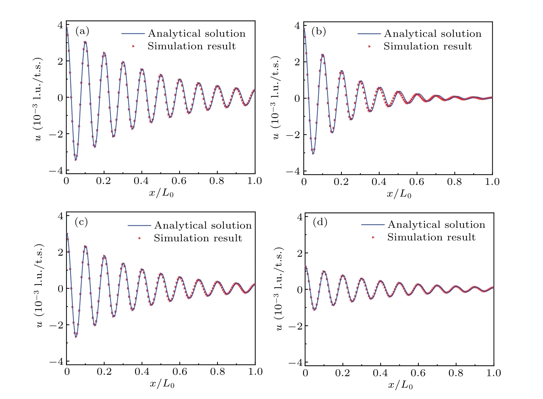
Fig.4. The sound attenuation simulation results.

4. Effect of viscosity on the stability and accuracy of MRT-LBM

Since the sound attenuation model is mainly studied by viscosity and density,the sound attenuation model can be used to test the numerical stability of the MRT model under extreme numerical conditions. From the comparative analysis of the density stability of SRT-LBM and MRT-LBM, it is apparent that the numerical stability of MRT-LBM is much better than that of SRT-LBM at low viscosity and high viscosity. This section continues to study further the influence of concentration,viscosity and density on the stability and accuracy of the MRT-LBM model based on the concept of the above attenuation channel model by considering the sound attenuation coefficient as an example.

In Subsections 4.1 and 4.2, we select four different density ratios,and then gradually change the value of the volume concentrationnσ. The purpose is to test whether the stability and accuracy of the MRT model under extreme viscosity will be significantly affected by changes in density ratio and volume concentration.

In Subsections 4.3 and 4.4, we fix the density ratio asρ1:ρ2=1:2. This part only changes the concentration ratio and mainly studies the influence of different viscosities on the stability and accuracy of the model.

4.1. Effect of low viscosity

The relaxation time in the SRT model is determined by fluid viscosity, and the diffusion coefficient determines the relaxation time for the convection-diffusion equation.[44-46]Therefore,for the relatively low fluid viscosity or the diffusion coefficient,the corresponding relaxation time approaches 0.5,and consequently the model becomes unstable numerically.

Under the condition ofμσ=νσandνσ=ν¯σ,the simulation results show that whenνσ ≤0.03,SRT-LBM is unstable.Therefore, in order to show the stability of MRT-LBM, we studied the error of the attenuation coefficient calculated by the MRT model at different concentrations and densities whenνσ=ν¯σ=0.01,0.02,0.03. For a two-component mixture,it is known thatn1+n2=1. Therefore,we set the concentration of one of the components, such asn1, from 0.1 to 0.9, then sincen2=1-n1,binary mixtures with different mixing ratios can be obtained.As shown in Tables 3(a)and 3(b),only the attenuation coefficient relative errorαewhenνσ=0.01 is listed.The variations in relative errorαewith different viscosities are displayed in Figs.5 and 6.

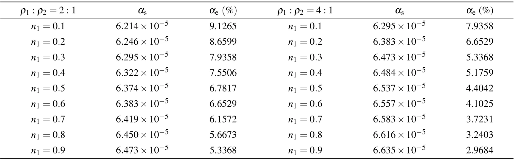
Table 3(a). The calculated results of the attenuation coefficient αs under different density ratios,and the viscosity is νσ =0.01. The relative errors αe between calculated results and analytical solutions are defined as αe=|(αs-α)/α|×100%.

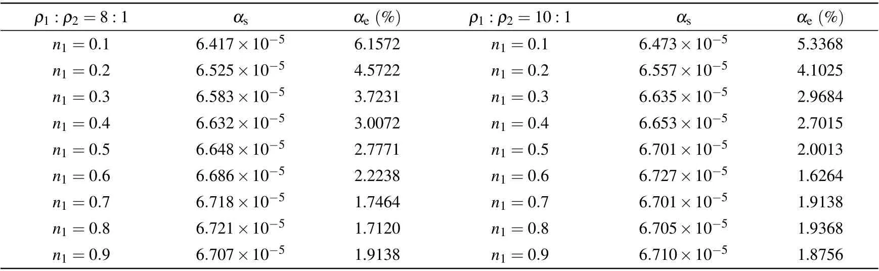
Table 3(b). The calculated results of the attenuation coefficient αs under different density ratios,and the viscosity is νσ =0.01.

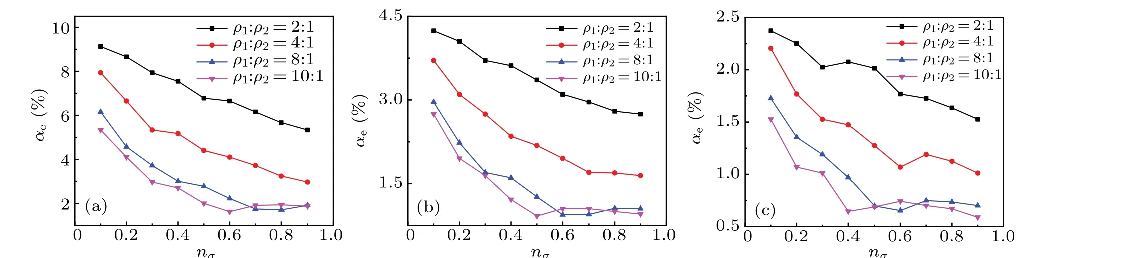
Fig.5. At low viscosity,the influence of concentration nσ and density ρσ on the relative error αe,when the viscosity is fixed to(a)ν1=ν2=0.01,(b)ν1=ν2=0.02,and(c)ν1=ν2=0.03.

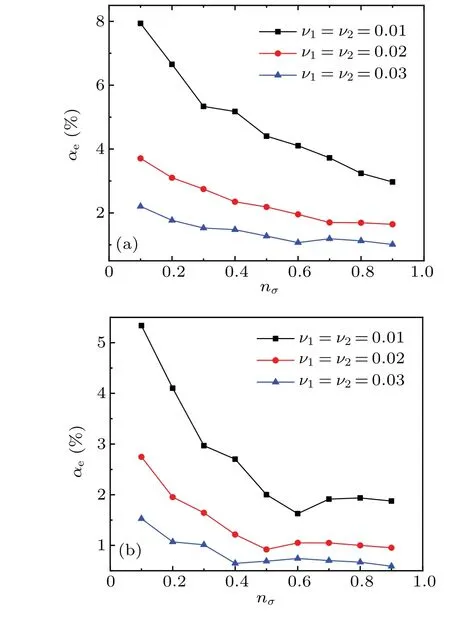
Fig. 6. Effect of low viscosity on the relative error αe, the density is (a)ρ1:ρ2=4:1 and(b)ρ1:ρ2=10:1.

As shown in Fig.5, as the viscosity value gradually increases fromνσ=0.01, the relative errorαebecomes significantly smaller. Whenνσ=0.03, the average relative error ¯αe=1.29%, which is much smaller than the average relative error ¯αe=4.44%whenνσ=0.01. In addition,if the viscosity is constant,it can be seen that for a two-component mixed gas,the increase in the concentration of the high-density component reduces the relative errorαe.and the concentration gradually increases from 0.1. It can be seen that when the viscosityνσ=ν¯σ=0.02,0.03,the accuracy of the model is improved as compared withνσ=0.01.From the perspective of the degree of change, when the viscosityνσ=ν¯σ=0.02,0.03,the relative error value changes smoothly with the concentration. When the viscosityνσ=0.01, the relative error changes relatively larger, but the average relative error ¯αe＜5%. Therefore, the results show that MRT-LBM has good numerical stability and calculation accuracy at low viscosity.

Figure 6 shows that the density ratio remains unchanged,

4.2. Effect of high viscosity

Similar to the above low viscosity case,a large fluid viscosity means a large relaxation time, and the no-slip boundary condition cannot be ensured.[42]This situation will have a greater impact on the stability of the model. The simulation results show that under the condition ofμσ=νσandνσ=ν¯σ,whenνσ ＞1.1,the SRT-LBM model is unstable. Similarly,in order to show the numerical stability of MRT-LBM at high viscosity,we studied the relative errorαecalculated by the MRT model whenνσ=ν¯σ=1.166,1.5. The calculation results are shown in Tables 4(a)and 4(b)and the variation in relative errorαewith different viscosities has been displayed in Fig.7.

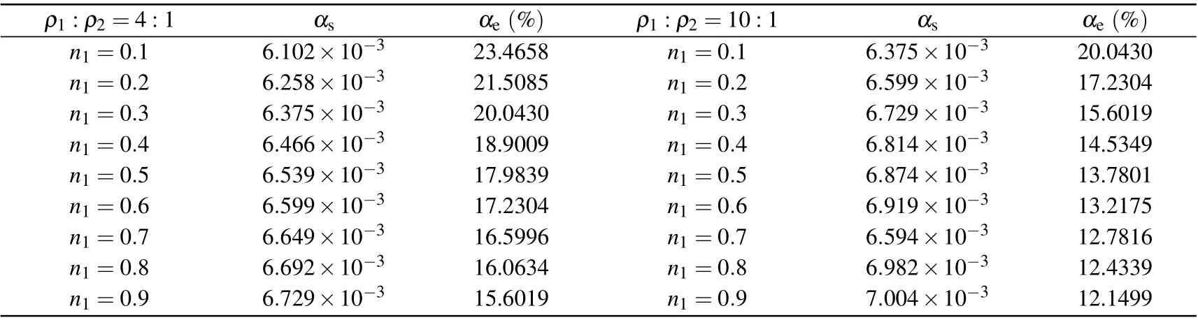
Table 4(a). The calculated results of the attenuation coefficient αs under density ratios ρ1 :ρ2 =4:1 and ρ1 :ρ2 =10:1 for the viscosity ν1=ν2=1.166.

According to Table 3(b),the density stability of the MRT model is affected when the viscosity is high. It can be considered that the density instability caused by the high viscosity makes the value of the relative errorαelarger. As shown in Fig.7,it is seen that when the viscosity is high,the calculation result of the relative errorαeremains stable under different viscosites and concentration ratios. From a numerical point of view, the average relative errors are 16.62% and 29.26% for the viscosity of 1.166 and 1.500,respectively. However,under this extreme viscosity, the SRT model is numerically unstable. Therefore,this can still show that the stability of the MRT model is better than that of the SRT model at high viscosity.In the future work, we will try to solve the problem of large relative errorαefrom different aspects.

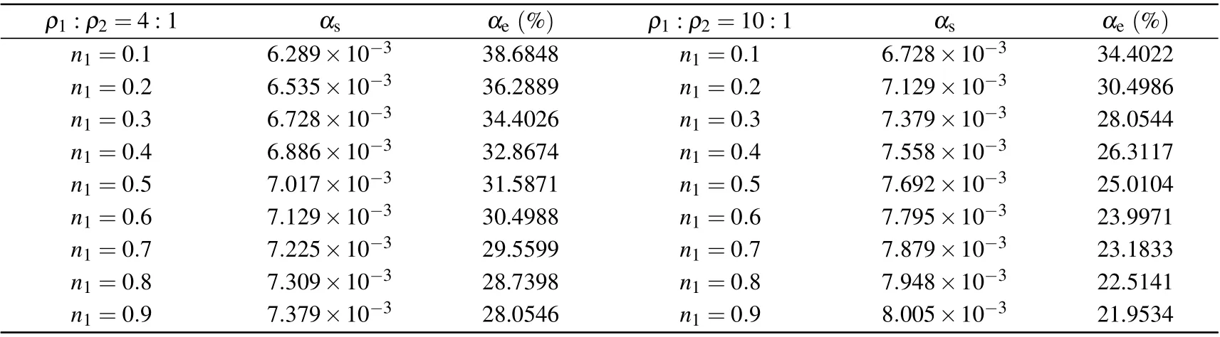
Table 4(b). The calculated results of the attenuation coefficient αs under density ratios ρ1 :ρ2 =4:1 and ρ1 :ρ2 =10:1, the viscosity is ν1=ν2=1.5.

Fig.7.Effect of high viscosity and density ratio on the relative error αe.

4.3. Model accuracy comparison at normal viscosity

Different from the previous two sections, it only calculates the relative errorαeof the MRT-LBM model at low viscosity and high viscosity. When the average shear viscosity is 0.03＜ν ≤1.1, the SRT-LBM model is stable. In order to compare the relative errors calculated by the two models under normal viscosity,we keep the density ratioρ1:ρ2=1:2 and gradually increase the viscosity. By comparing the simulation results of the two models,we find that the relative errors are the same. Therefore, Table 5 only lists the relative errors of the MRT model corresponding to the viscosity difference|ν1-ν2|=0.1. The variation in relative errorαewith different viscosities has been displayed in Fig.8.

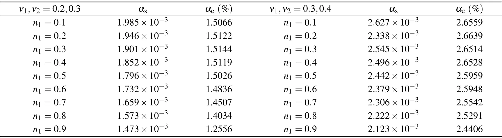
Table 5. Under the condition of μσ =νσ,the relative error αe calculated by MRT-LBM.

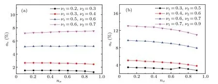
Fig.8. Effect of normal viscosity on the relative error αe.

By comparing the calculation results of the relative error,it can be seen that the accuracies of SRT-LBM and MRT-LBM are completely consistent with each other under normal viscosity. Therefore, it is difficult to reflect the advantages of MRT model calculation accuracy. However, it reflects from the side that the MRT model has increased the scope of application without reducing its accuracy. Only the MRT-LBM simulation results are shown in Fig.8. Under normal viscosity conditions,the MRT model has excellent stability,and the change of concentration ratio has little effect on the result of relative error.

The above three sections are divided according to the different viscosites. It can be seen that the SRT model is unstable at low and high viscosities,and the MRT model has excellent stability. In other words,the presented MRT model improves the stability under extreme viscosity conditions, so the MRT model has a wider application range. In order to illustrate the rationality of verifying the stability of the MRT model through the sound attenuation model,we study the impact of the error term of the macroscopic equation on the MRT model.

4.4. Effect of the error term of the macroscopic equation on accuracy

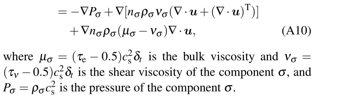
Through C-E analysis, the macroscopic and momentum conservation equations of MRT-LBM can be restored. However, comparing Eq. (A1) and Eq. (A2), we can see that the conservation condition is affected by the bulk viscosityμσand the shear viscosityυσ. The specific error expression is∇ρ(μ-ν)∇·u. It can be seen that the viscosity difference(μ-ν) has a significant effect on the above expression. In order to verify the impact of the error term of the macroscopic equation,the viscosity difference is defined as Δν=(μ-ν),the value of the viscosity difference Δνranges from 0.1 to 0.9, and the average value of viscosity (μ+ν)/2 is kept unchanged. The average value of viscosity is respectively taken as(μ+ν)/2=0.5,0.6,0.7 and 0.8. The density ratio remainsρ1:ρ2=1:2,and the concentration ratio isn1:n2=5:5.The calculated values ofαeand error Δαare shown in Table 6(a)and Table 6(b).

The error Δαis defined as Δα=|αe-α¯e|,which represents the difference between the relative error calculated under the conditions ofμ/=νandμ=ν. The expression of relative errorα¯eis the same as that ofαe. However,forμ/=ν,α¯erepresents the relative error calculated when the viscosity is set toμ=ν=(μ+ν)/2. This setting can make the attenuation coefficient have the same analytical solution,so that the error Δαcan be obtained by direct subtraction.

In Fig. 9(a), the four lines are almost parallel. It can be seen that the viscosity difference has almost the same effect on the different components. Figure 9(b)shows the influence of the viscosity difference Δνon the error Δα. The following three conclusions can be obtained: (a)When the viscosity difference is small, the error Δαis close to 0. (b) The error Δαhas nothing to do with the average viscosity value. (c)The error Δαis positively correlated with the viscosity difference Δν.

In fact,the error Δαis caused by the expression ∇ρ(μν)∇·u. Then the following two conclusions can be obtained.First of all,the calculation result of the error Δαcan correctly reflect the influence of the expression ∇ρ(μ-ν)∇·u.In otherwords, the above calculation can reflect the impact of the error term of the macroscopic equation. Secondly,it also shows that this paper uses the relative error of the attenuation coefficient as an example to explore the stability and accuracy of MRT-LBM, offering a certain degree of universality. This means that the MRT model should have similar stability and accuracy when applied to other problems.

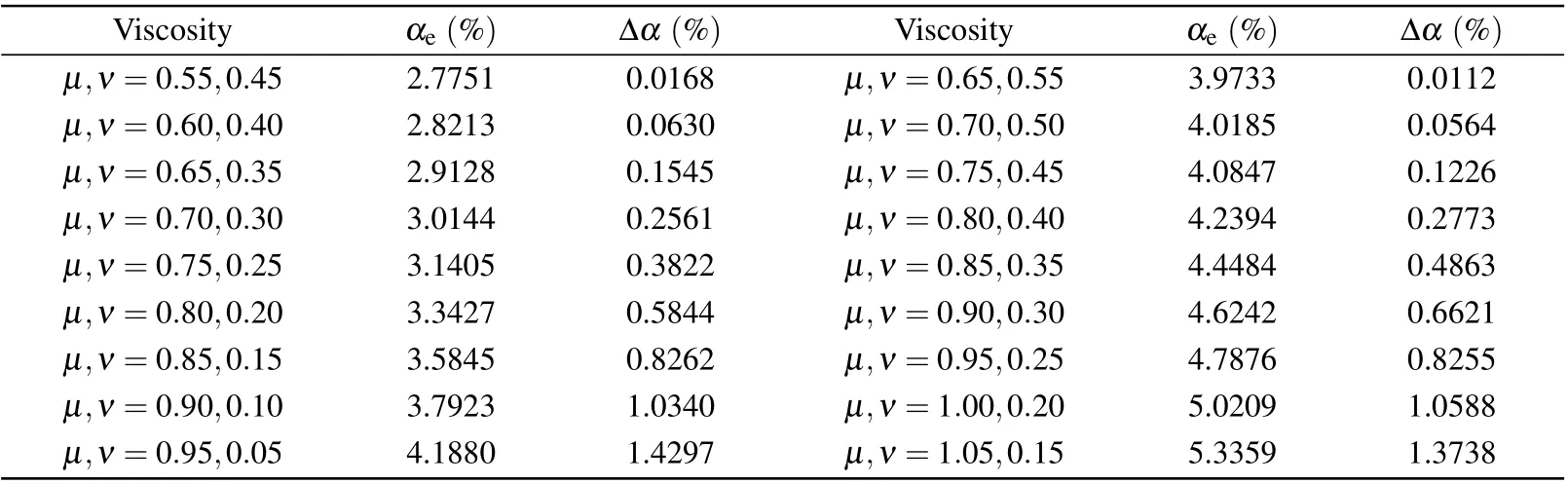
Table 6(a). Under the condition of μ /=ν. The average value of viscosity(μ+ν)/2=0.5,0.6,and the Δν ranges from 0.1 to 0.9.

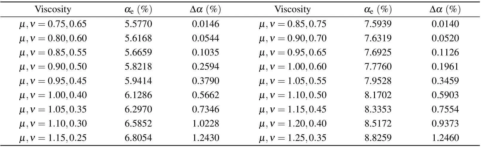
Table 6(b). Under the condition of μ /=ν. The average value of viscosity is(μ+ν)/2=0.7,0.8,and the Δν ranges from 0.1 to 0.9.

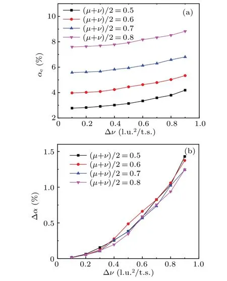
Fig. 9. (a) Effect of viscosity difference Δν on relative error αe. (b)Effect of viscosity difference Δν on error Δα.

5. Conclusion

In summary,an improved LBM model has been incorporated with the MRT collision operator to verify the attenuation of sound waves through the binary mixtures of gas. The sound attenuation process is closely related to viscosity,macroscopic velocity and density.Therefore,we use the relative error of the sound attenuation coefficient to study the influence of viscosity on the accuracy and stability of the MRT-LBM model. The macroscopic and the momentum conservation equations of the MRT model are obtained through the CE expansion analysis.In order to verify that the MRT model is suitable for simulating two-component flow problems, the model has been used to simulate the diffusion phenomenon. Then we have verified the stability of the MRT model and applied the model to the study of sound attenuation characteristics in binary gas mixtures. Different viscosities have a significant impact on model stability and calculation accuracy. Therefore,intensive research has been carried out according to the difference in viscosity. Several conclusions can be drawn as follows.

(1) The effect of low viscosity. When the average shear viscosityνis close to 0,the SRT model is numerically unstable, and the present MRT model can still maintain numerical stability with high calculation accuracy.

(2)The effect of high viscosity. Similar to low viscosity,when the average shear viscosityν ＞1.1,the value calculated by using the SRT model is unstable.However,from this investigation,the value of the MRT model remains stable,but with less accuracy.

(3) For the average shear viscosity in the range 0.03＜ν ≤1.1, the values calculated through both SRT model and MRT models remain stable. The simulation results show that the calculation accuracies of the two models are exactly the same under different concentrations and density ratios. Under normal viscosity, the SRT model and the MRT model remain stable,and concentration changes have little effect on stability.

(4)The above studies all maintainμ=ν,we setμ/=νto study the impact of the error term of the macroscopic equation on the accuracy and stability of the model. According to the expression ∇ρ(μ-ν)∇·u, this paper mainly studies the influence of the viscosity difference on the error Δα. The results show that the error Δαhas nothing to do with the viscosity value while it is positively correlated with the viscosity difference. When the viscosity difference is relatively small,the error Δαapproaches 0. It is found that the simulation result is consistent with the conclusion reflected by the expression∇ρ(μ-ν)∇·u. At the same time, this also shows that the conclusions about the stability of the model drawn from the relative error of the attenuation coefficient has a certain general applicability.

The outcome of this research indicates that the improved model used in this study can be applied for solving a variety of binary mixture fluid flows with achieving the high numerical stability. Hence, the model developed in this study may have a broad application prospect. The sound attenuation model is used to study the stability of the MRT model, which provides a method to verify the stability of the LBM model. The current research is mainly focused on the stability and accuracy of the model itself. Our future work aims to extend the application of the current model to study non-premixed and multi-component fluids with high viscosity and density ratios.

Acknowledgements

Project supported by the National Natural Science Foundation of China (Grant Nos. 12174085, 11874140,and 11574072), the State Key Laboratory of Acoustics, Chinese Academy of Sciences(Grant No.SKLA201913),and the Postgraduate Research and Practice Innovation Program of Jiangsu Province,China(Grant No.KYCX210478).

Appendix: Chapman-Enskog analysis of thepresent MRT model

The macroscopic equation and the momentum conservation equation can be derived from Eq. (1) through the Chapman-Enskog (C-E) expansion analysis, (εis the Knudsen number)and the multi-scale expansion is as follows: