马学敏, 张怀德, 李宝麟

(1- 甘肃中医药大学理科教学部，定西 743000; 2- 西北师范大学数学与信息科学学院，兰州 730070)

Measure differential equations have been considered by many authors[1-5]. Measure functional differential equations represent a special class of measure differential equations[6,7]. There are many sources described the class of equations in recent years,such as[8-12]. Especially,in[4,12],the author stated very nice stability results of measure differential equations. But they discussed the quasi equi-asymptotical stability,exponential stability and variational stability. Here we discuss Φ-variational stability for measure functional differential equations with infinity delay by using the bounded Φ-variation function. The Lyapunov type theorem for the Φ-variational stability and asymptotically Φ-variational stability of the bounded Φ-variational solutions are established. These results are essential generalization of the results in [12].

1 Introduction

Measure differential equations have been considered by many authors[1-5]. Measure functional differential equations represent a special class of measure differential equations[6,7]. There are many sources described the class of equations in recent years,such as[8-12]. Especially,in[4,12],the author stated very nice stability results of measure differential equations. But they discussed the quasi equi-asymptotical stability,exponential stability and variational stability. Here we discuss Φ-variational stability for measure functional differential equations with infinity delay by using the bounded Φ-variation function. The Lyapunov type theorem for the Φ-variational stability and asymptotically Φ-variational stability of the bounded Φ-variational solutions are established. These results are essential generalization of the results in [12].

In this paper, we consider the stability of the bounded Φ-variation solution to measure functional differential equations of the form

where Dx, Du denote the distributional derivative of function x and u. x is an unknown function with values in Rnand the symbol xtdenotes the function xt(τ) = x(t+τ)defined on (-∞,0], which is corresponding to the length of the delay. The function f,g : [t0,t0+σ]×P →Rn, u : [t0,t0+σ] →R is a nondecreasing and continuous function from the left, where

P ={xt:x ∈O,t ∈[t0,t0+σ]}⊂H0, H0⊂X((-∞,0],Rn)

Our candidate for the phase space of measure functional differential equations with infinity delay is a linear space H0⊂X((-∞,0],Rn) equipped with a norm denoted by‖·‖*. It is assumed that this normed linear space H0satisfies the following conditions:

(H1): H0is complete;

(H2): If x ∈H0and t ＜0, then xt∈H0;

(H3): There exists a locally bounded function k1: (-∞,0] →R+such that if x ∈H0and t ≤0, then ‖x(t)‖≤k1(t)‖x‖*;

(H4): There exists a function k2:(0,∞)→[1,∞) such that if σ ＞0 and x ∈H0is a function whose support is contained in[-σ,0], then‖x‖*≤k2(σ)supt∈[-σ,0]‖x(t)‖;

(H5): There exists a locally bounded function k3: (-∞,0] →R+such that if x ∈H0and t ≤0, then ‖xt‖*≤k3(t)‖x‖*;

(H6): If x ∈H0, then the function t →‖xt‖*is regulated on (-∞,0].

This paper is organized as follows: in the next section, we show some basic definitions and lemmas. In the final section, we prove an important inequality which will be used for obtaining the main results of this paper firstly. After that, we obtain the theorems of Φ-variational stability and asymptotically Φ-variational stability for measure functional differential equations with infinity delay.

2 Main definitions and lemmas

In this section, we will show some basic definitions and lemmas. First let’s start with the definition of Kurzweil integral and FΦ([t0,t0+σ]×P,h,ω).

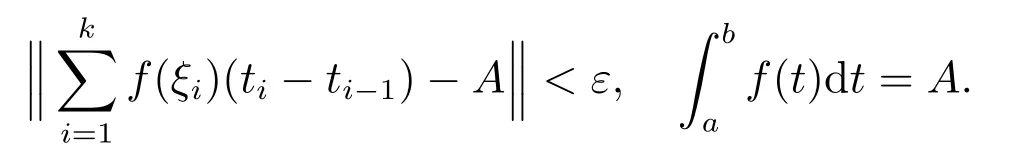
Definition 1[13]Let f : [a,b] →Rnbe a function. f is said to be Kurzweil integrable to A on [a,b] if for every ε ＞0, there exists a positive function δ(ξ) such that whenever a division D given by a=t0＜t1＜···＜tk=b,and any{ξ1,ξ2,··· ,ξk},satisfies ξi-δ(ξi)＜ti-1≤ξi≤ti＜ξi+δ(ξi) for i=1,2,··· ,k. We have

Let Φ(u)denote a continuous and increasing function defined for u ≥0 with Φ(0)=0, Φ(u)＞0 for u ＞0, and satisfying the following conditions:

(Δ2): There exist u0≥0 and a ＞0 such that Φ(2u)≤aΦ(u) for u0≥u ＞0;

(c): Φ(u) is a convex function.

We consider the function x:[a,b]→Rn, x(t) is of bounded Φ-variation over [a,b]if for any partition π :a=t0＜t1＜···＜tm=b, we have

VΦ(x;[a,b]) is called Φ-variation of x(t) over [a,b].

Definition 2 A function g :[t0,t0+σ]×P →Rnbelongs to the class FΦ([t0,t0+σ]×P,h,ω) if:

(i) There exists a positive function δ(τ) such that for every [m,n] satisfy τ ∈[m,n]⊂(τ -δ(τ),τ +δ(τ))⊂[t0,t0+σ] and xτ∈P, we have

(ii) For every [m,n] satisfy τ ∈[m,n] ⊂(τ -δ(τ),τ +δ(τ)) ⊂[t0,t0+σ] and xτ,yτ∈P, we have

where h : [t0,t0+ σ] →R is nondecreasing function and continuous from the left.ω : [0,+∞) →R is a continuous and increasing function with ω(0) = 0, ω(ar) ≤aω(r), ω(r)＞0 for a ＞0, r ＞0.

For obtaining main results, let us introduce some concepts of the trivial solution x(s)=0, s ∈[0,+∞) of the equation (1).

Definition 3 The solution x ≡0 of(1)is called Φ-variationally stable if for every ε ＞0 there exists δ = δ(ε) ＞0, such that if y : [t0,t1] →Rn, 0 ≤t0＜t1＜+∞is a function of bounded Φ-variation on [t0,t1], continuous from the left on (t0,t1] with Φ(‖y(t0)‖)＜δ, and

then we have

Φ(‖y(t)‖)＜ε, t ∈[t0,t1].

Definition 4 The solution x ≡0 of(1)is called Φ-variationally attracting if there exists δ0＞0, and for every ε ＞0, there is a T =T(ε)＞0 and γ =γ(ε)＞0 such that if y : [t0,t1] →Rn, 0 ≤t0＜t1＜+∞is a function of bounded Φ-variation on [t0,t1],continuous from the left on (t0,t1] with Φ(‖y(t0)‖)＜δ0, and

then

Φ(‖y(t)‖)＜ε, ∀t ∈[t0,t1]∩[t0+T(ε),+∞), t0≥0.

Definition 5 The solution x ≡0 of (1) is called Φ-variationally-asymptotically stable, if it is Φ-variationally stable and Φ-variationally attracting.

Lemma 1[14]If H0⊂X((-∞,0],Rn)is a space satisfying conditions(H1)-(H6),then the following statements are true for every a ∈R.

1) Hais complete.

2) If x ∈Haand t ≤a, then xt∈Ha.

3) If t ≤a and x ∈Ha, then ‖x(t)‖≤k1(t-a)‖x‖*.

4) If σ ＞0 and x ∈Ha+σis a function whose support is contained in [a,a+σ],then ‖x‖*≤k2(σ)supt∈[a,a+σ]‖x(t)‖.

5) If x ∈Ha+σand t ≤a+σ, then ‖xt‖*≤k3(t-a-σ)‖x‖*.

6) If x ∈Ha+σ, then the function t →‖xt‖*is regulated on (-∞,a+σ].

Lemma 2[15]Assume that -∞＜a ＜b ＜+∞and that f,g : [a,b] →R are functions which are continuous from the left in [a,b].

If for every σ ∈[a,b], there exists δ(σ) ＞0 such that for every η ∈(0,δ(σ)) the inequality

f(σ+η)-f(σ)≤g(σ+η)-g(σ)

holds, then

f(s)-f(a)≤g(s)-g(a), ∀s ∈[a,b].

3 Φ-variational stability

In this section, we prove an important inequality which will be used for obtaining the main results of this paper firstly.

Theorem 1 Suppose that V :[0,+∞)×Rn→R, is such that for every x ∈Rn,the function V(·,x) : [0,+∞) →R is continuous from the left in (0,+∞). Assume that:

(i)

for x,y ∈Rn, t ∈[0,+∞) with a constant L ＞0;

(ii) Further assume that there is a real function H : Rn→R such that for every solution x : (α,β) →Rnof the measure functional differential equation (1) on(α,β)⊂[0,+∞), we have

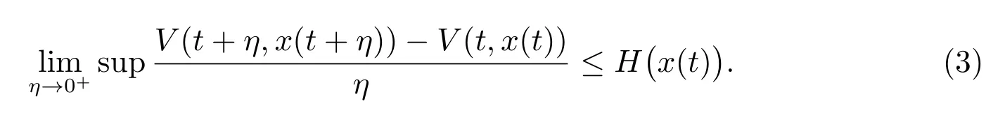
If y :[t0,t1]→Rn, 0 ≤t0＜t1＜+∞is continuous from the left on (t0,t1] and of bounded Φ-variation on (t0,t1], then the inequality

Proof Let y : [t0,t1] →Rnbe a function bounded Φ-variation and continuous from the left on(t0,t1]. It is clear that the function V(t,y(t)):[t0,t1]→R is continuous from the left on (t0,t1].

Let σ ∈[t0,t1] be an arbitrary point, assume that x : [σ,σ +η1(σ)] →Rnis a solution of bounded Φ-variation on [σ,σ +η1(σ)], η1＞0 with the initial condition x(σ)=y(σ) and xσ=yσ. The existence of such a solution is guaranteed in the paper[14]. Furthermore, the measure functional differential equations with delay have the form

Dx=f(s,xs)+g(s,xs)du(s)

is equivalent to the following form

by [14]. Then

exist, by (2), we have

for every η ∈[0,η1(σ)].

By this inequality and by (3) we obtain

where ε ＞0 is arbitrary and η ∈(0,η2(σ)) with η2(σ) ≤η1(σ), η2(σ) is sufficiently small.

Define

The function Ψ : [t0,t1] →Rnis continuous from the left on (t0,t1] of bounded Φvariation on [t0,t1], and by Theorem 1.02, Theorem 1.11 and Theorem 1.17 in the paper[16], the last inequality can be used to derive

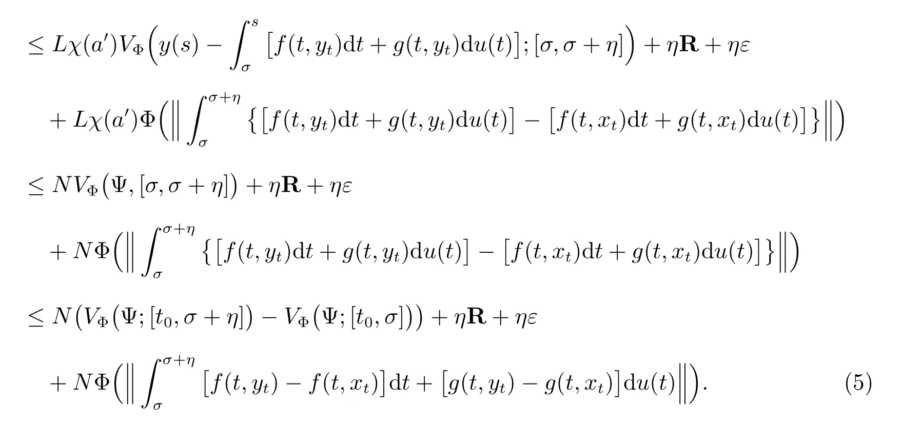
Let us consider the last term in (5). Since f,g ∈FΦ([t0,t0+ σ] × P,h,ω) for every ε ＞0, there exists a positive function δ : [σ,σ + η] →(0,+∞), such that whenever a δ-division D of [σ,σ+η] given by D = {(τj;[αj-1,αj]),j = 1,2,··· ,m},let M(t) = VΦ(h;[σ,t]), σ ≤t ≤σ+η, by the definition of Φ(u) and h, then M(t) is nonnegative, nondecreasing and continuous from the left, we have

for ρ ∈[σ,σ+η2(σ)], we have

so

Consequently

For every ε ＞0, we define

for ρ ∈(σ,σ+η3(σ)) and also

Let us denote

Since Ψ is of bounded Φ-variation on [t0,t1], the set P(β) is definite and we denote by n(β) the number of elements of P(β). If σ ∈[t0,t1]P(β) and ρ ∈(σ,σ+η3(σ)), then by (9), we have

Because k3is a locally bounded function, there exists A ＞0, such that k3(t-σ-η)·k2(η)≤A. Further, we have

So when η ∈(0,η3(σ)), by (6), we have

If σ ∈[t0,t1]∩P(β),then there exists η4(σ)∈(0,η3(σ))such that for η ∈(0,η4(σ)),we have

and (σ,σ+η4(σ))∩P(β)=Ø. Hence (6) and (9) yield

Define now

If σ ∈[t0,t1]P(β), then set δ(σ) = η3(σ) ＞0; and if σ ∈[t0,t1]∩P(β), then set δ(σ) = η4(σ) ＞0; for σ ∈[t0,t1], η ∈(0,δ(σ)), by (10),(11) and by the definition of Mα, we obtain the inequality

Therefore by Theorem 1.03, Theorem 1.17 in [3], we have

So when σ ∈[t0,t1], η ∈(0,δ(σ)), by (5), we have

where

G(t)=N(VΦ(Ψ;[t0,t]))+R(t-t0)+ε(t-t0)+NVΦ(Mα;[t0,t]),

G is continuous from the left on [t0,t1]. By Lemma 2 and (13),(14), we obtain

Since ε ＞0 can be arbitrarily small, we obtain from this inequality the result given in(4).

In the following, we obtain the theorems of Φ-variational stability and asymptotically Φ-variational stability for measure functional differential equations with infinite delay.

(i) There exists a continuous increasing real function v :[0,+∞)→R such that v(ρ)=0 ⇔ρ=0;

(ii)

L ＞0 being a constant

If the function V(t,x(t))is non increasing along every solution of the equation(1),then the trivial solution of (1) is Φ-variationally stable.

Proof Since we assume that the function V(t,x(t)) is non increasing whenever x(t):[α,β]→Rnis a solution of (1), we have

Let us check that under these assumptions the properties required in Definition 3 are satisfied.

Let ε ＞0 be given and let y : [t0,t1] →Rn, 0 ≤t0＜t1＜+∞be of bounded Φ-variation on [t0,t1] and continuous from the left in (t0,t1]. Since the function V satisfies the assumptions of Theorem 1 with H ≡0 in the relation (3). We obtain by(4),(16),(17) the inequality

which holds for every r ∈[t0,t1].

Let us define α(ε)=infr≤εv(r), then α(ε)＞0, infε→0+α(ε)=0. Further, choose δ(ε) ＞0 such that 2Nδ(ε) ＜α(ε). If in this situation the function y is such that Φ(‖y(t0)‖)＜δ(ε), and

then by (18), we obtain the inequality

provided r ∈[t0,t1].

which contradicts (19).

Hence Φ(‖y(t)‖) ＜ε for all t ∈(t0,t1], and by Definition 3 the solution x ≡0 is Φ-variationally stable.

holds for every t ∈[t0,t1], where H :Rn→R is continuous, H(0)=0, H(x)＞0(x/=0), then the solution x ≡0 of (1) is Φ-variationally-asymptotically stable.

Proof From (20) it is clear that the function V(t,x(t)) is non increasing along every solution x(t) of (1) and therefore by Theorem 2 the trivial solution x ≡0 of (1)is Φ-variationally stable.

By Definition 5 it remains to show that the solution x ≡0 of (1) is Φ-variationally attracting in the sense of Definition 4.

From the Φ-variational stability of the solution x ≡0 of(1)there is a δ0∈(0,Φ(a)),such that if y : [t0,t1] →Rnis of bounded Φ-variation on [t0,t1], where 0 ≤t0＜t1＜+∞, y is continuous from the left on (t0,t1] and such that Φ(‖y(t0)‖)＜δ0, and

Let ε ＞0 be arbitrary. From the Φ-variational stability of the trivial solution we obtain that there is a δ(ε) ＞0, such that for every y : [t0,t1] →Rnis of bounded Φ-variation on [t0,t1], where 0 ≤t0＜t1＜+∞, y is continuous from the left on (t0,t1]and such that Φ(‖y(t0)‖)＜δ(ε), and

we have Φ(‖y(t)‖)＜ε, for t ∈[t0,t1].

Let

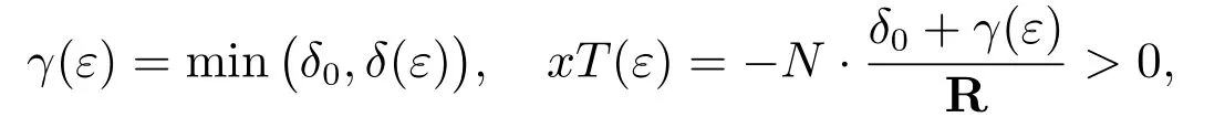
where

R=sup{-H(x):γ(ε)≤Φ(‖x‖)＜ε}=-inf{H(x):γ(ε)≤Φ(‖x‖)＜ε}＜0.

Assume that y :[t0,t1]→Rnis of bounded Φ-variation on [t0,t1], continuous from the left on (t0,t1] and such that Φ(‖y(t0)‖)＜δ0, and

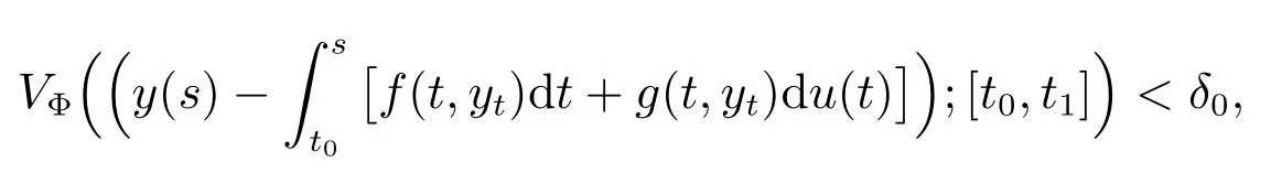
Assume that T(ε) ＜t1-t0, i.e. t0+T(ε) ＜t1. We show that there exists a t*∈[t0,t0+T(ε)] such that Φ(‖y(t*)‖)＜γ(ε). Assume the contrary, i.e. Φ(‖y(s)‖)≥γ(ε),for every s ∈[t0,t0+T(ε)]. Theorem 1 yields

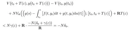
Hence

V(t0+T(ε),y(t0+T(ε)))≤V(t0,y(t0))-Nδ0≤LΦ(‖y(t0)‖)-Nδ0≤NΦ(‖y(t0)‖)-Nδ0＜(N -N)δ0=0,

and this contradicts the inequality

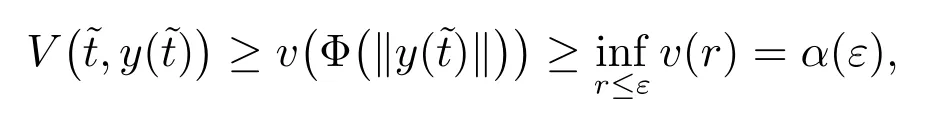
V(t0+T(ε),y(t0+T(ε)))≥v(Φ(‖y(t0+T(ε))‖))≥v(γ(ε))＞0.

Hence necessarily there is a t*∈[t0,t0+T(ε)] such that Φ(‖y(t*)‖) ＜γ(ε). And by(21), we have Φ(‖y(t)‖) ＜ε, for t ∈[t*,t1]. Consequently, also Φ(‖y(t)‖) ＜ε, for t ＞t0+T(ε), and therefore the trivial solution x ≡0 is a variationally attracting solution of (1).

Remark 1 If the function Φ(u) defined in section 2 satisfies

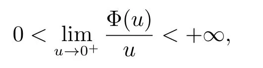
then by Theorem 1.15 of [16], BVΦ[a,b]=BV[a,b], where BV[a,b] represents the class of all functions of bounded variation in usual sense on[a,b]. Therefore,in this case,the results of Theorem 1, Theorem 2 and Theorem 3 are equivalent to the results in [12].Notice that if

by Theorem 1.15 of [16], we have

BV[a,b]⊂BVΦ[a,b].

For example Φ(u)=up(1 ＜p ＜∞), we have

Therefore, Theorem 2 and Theorem 3 are essential generalization of the results in [12].