滕冠兴，戚俊毅，葛 昊，李 哲，张剑波，2

（1清华大学汽车安全与节能国家重点实验室，北京100084；2北京理工大学北京电动汽车联合创新中心，北京100081）

Lithium-ion batteries (LIBs) have become the mainstream energy storage system for propulsion of electric vehicles due to their high voltage, high energy density, long life span and low self-discharging rate.The performance, degradation, and safety of LIBs are sensitive to temperature and hence thermal design and management of LIBs are of paramount importance in vehicular application[1-4]. Thermal modeling can speed up the optimization of cell design and battery management. The governing equation for the thermal behavior of LIBs reads,

where ρ is the density, Cpthe specific heat capacity, T the temperature, k the thermal conductivity and q the heat generation rate of the cell. Thermal parameters, namely, the specific heat capacity and the thermal conductivity, determine the reliability and accuracy of thermal modeling[5].As a result, accurate estimation of thermal parameters is an issue of central importance in thermal modeling, which is though very challenging. First, each cell is composed of multiple layers with different thermal properties, hence,thermal parameters are intrinsically anisotropic.Notably, parallel and perpendicular (axial and radial)thermal conductivities should be distinguished for laminated(spiral-wound)cells.Second,the cell core is soaked with the electrolyte, causing the thermal properties to be different from the dry state and hence additional difficulties in estimating them; in-situ estimation is therefore required. Third, the cell core is encased by a layer of Al-plastic film, the thermal properties of which differs greatly from that of the core.In a word,the cell is by no means homogenous.

There are several approaches of varied complexities and accuracies to estimate the thermal parameters of LIBs. At the first approximation, the ensemble average method calculates a mass average value of components with thermal parameters known as prior[6-9]. This approach has been proved to estimate the specific heat capacity with an acceptable accuracy, as calibrated with more accurate methods such as accelerating rate calorimeter (ARC) and isothermal battery calorimeter (IBC) [10]. Yet it severely overestimated the thermal conductivity. This discrepancy has its root in the fact that thermal contact resistance and electrolyte wetting environment is not taken into consideration[11].

To overcome the difficulties in estimating the thermal conductivity, the xenon flash technique (XFT)[12] and transient plane source (TPS) methods[13] are proposed. These two methods suffer from several limitations, notably that they treat the LIB as a homogeneous object, which is at odds with the fact that the LIB has highly heterogeneous features, e.g.,the cell is made of multiple layers with distinct thermal properties in different directions. Moreover,they both need a known specific heat capacity as an input, which, nevertheless, is not always known and hence introduces additional errors.

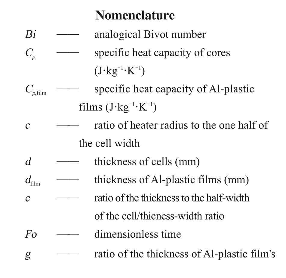
To address these limitations, we developed a new method, termed modified transient plane source(MPTS) method, which is able to estimate multiple thermal parameters simultaneously via a combined experimental and computational approach[5]. In this method, as shown in Figure 1, a circular planar heater is sandwiched by two cells under approximately adiabatic environment. Thermocouples are placed at multiple predefined locations on the cell surface. The cells are heated for a duration of time and the temperatures at the thermocouples are recorded. To extract thermal parameters from experimental data, a 2D axisymmetric thermal model capturing key features of LIBs including the Al-film encasing and the contact thermal resistance between the casing and the cell cores is employed, and optimization methods are used to estimate the parameters simultaneously.Table 1 summarizes the features of the methods.

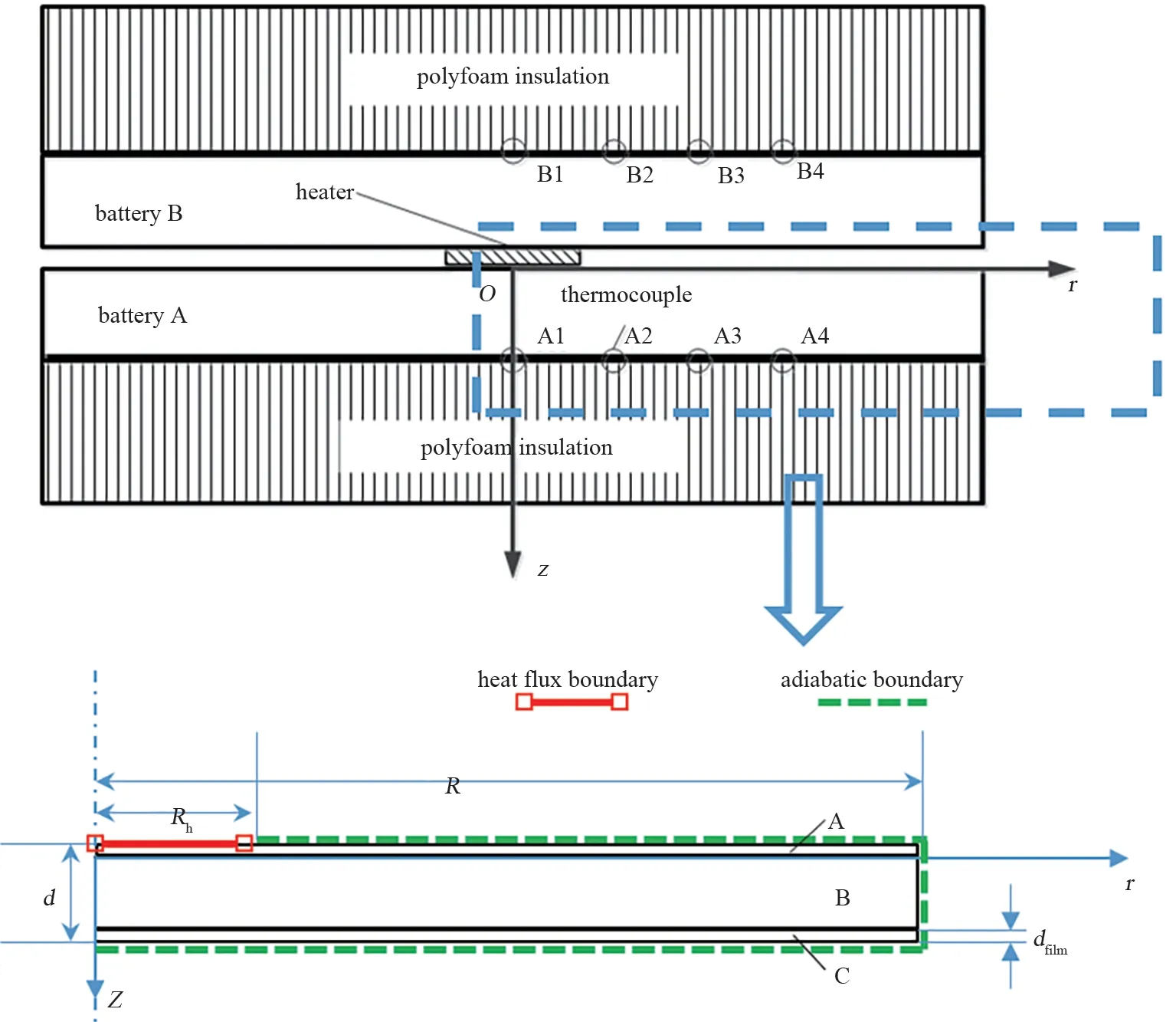
Fig.1 Schematic diagram of the experimental setup and the model.A circular heater is sandwiched by two cells.Poly‐foam is used to cover the cells for creating approximately adiabatic environment.Thermocouples are attached at multi‐ple deliberately-chosen locations on the cell surface.The cells are heated for a duration of time and the corresponding temperature evolution is recorded.In the model,the r and z axis are in-plane and though-plane directions of the LIBs,respectively.The origin locates at the center of the circular heater.Domain A and C represent the Al-plastic films enfold‐ing the cell core,denoted as Domain B,composed of electrolyte soaked electrodes and separators

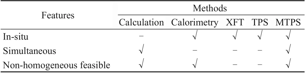
Table 1 The comparison of methods for thermal parameters estimation

The MTPS method was validated by other methods[14-15], and our results are also referred to by other groups[16-20]. In our previous work, the parameter sensitivity was examined using the dimensional governing equations. Such results only hold to the specific dimension of the cell used in that paper. When the MTPS method is to be applied to a cell with different dimension, the corresponding sensitivity has to be checked again. In contrast, if non-dimensional governing equations are used in parameter sensitivity analysis, the obtained results apply to all the cases satisfying the similarity criteria. This general applicability of the results will be more valuable to the practitioners estimating LIB thermal parameters.

The purpose of this paper is to systematically study the precision of the MTPS method through the sensitivity analysis using non-dimensional equations,trying to identify the key experimental conditions determining the resolution of the method. Specifically,the radius and the power of the heater, the placement of thermocouples and the heating protocol, etc., will be examined. Understandings of these effects will facilitate the application of MTPS method at desired precision.

The remainder of this paper is organized as follows. Section two presents the model development,namely the governing equations and boundary conditions of the 2D axisymmetric numerical thermal model used in MTPS method, followed with model nondimensionalization which is a new development here. Section three discusses how the experimental conditions affect the estimation precision of the MTPS method, resulting in several general principles for optimizing the experimental setup and detailed analysis on the applicability of the MTPS method,which are major contribution of this paper. Section four concludes the paper.

1 Methodology

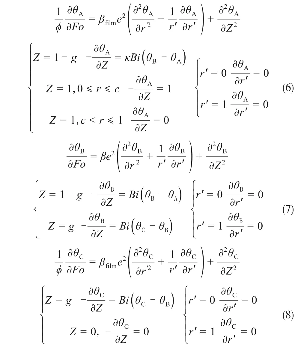
In MTPS method, the diameter of the disk heater is one order of magnitude smaller than the cell width.Hence, the temperature is symmetrically distributed before the edge of the cell takes effect on the temperature field, which will lead to the failing of the 2D axisymmetric assumption of the thermal model,and then a 2D axisymmetric thermal model is adopted to simulate the temperature distribution in this work,which reduce the computational overhead, as shown in Figure 1.The r and z axis are in-plane and though-plane directions of the LIBs, respectively. The origin locates at the center of the circular heater. Domain A and C represent the Al-plastic films encasing the cell core,denoted as Domain B, composed of electrolyte-soaked electrodes and separators. The governing equations and boundary conditions of the model are given by,

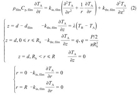
for the domain A,and,

for the domain B,and,

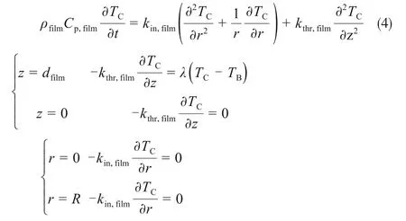
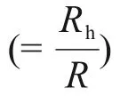
for the domain C. Equations (2)～(4) are also mentioned in our previous work[1]. Terms with the subscript of film correspond to the Al-plastic film.d is the thickness of the whole cell in m. ρ is the mass density in kg·m-3. Cpis the specific heat capacity in J·kg-1·K-1. kinand kthrare the parallel (in-plane) and perpendicular (through-plane) thermal conductivities in W·m-1·K-1, respectively. λ is the thermal conductance between the core and the film in W·m-2·K-1. q is the heat flux in W·m-2. P is the applied power to samples in W. R is the radius of the axisymmetric 2D model in m, which is equal to one half of the cell width. Rhis the radius of the circular heater in m.T is the temperature solution to Eq. (2)～(4) in K. T0is the initial temperature of the whole experimental system.

1.1 Model nondimensionalization

The model is now subjected to nondimensionalization for the sake of generalization and simplification. Below are dimensionless variables to be used in later development

where θ is the dimensionless temperature,r’and Z are the dimensionless spatial coordinate, e is the thickness-width ratio defined as the thickness d divided by R, c is the ratio of heater radius Rhto R, g is the ratio of the thickness of the Al-plastic film to the cell thickness,Fo is the dimensionless time, β, κ, φ and Bi are four dimensionless thermal parameters corresponding to kin,kthr,Cpand λ,respectively.β is the dimensionless in-plane thermal conductivity relative to the through-plane counterpart, named as thermal conductivity ratio in this paper.

Given above definitions, Eq. (2) ～(4) are transformed to,

Equation (6)～(8) are not amenable to analytical solutions. As a result, we resort to numerical solution below. Now, we can write the dimensionless temperature solution θ to Eq.(6)～(8)as follows,

Note that θ is independent of the heat flux q but determined by the intrinsic characteristics of the system, instead. The dimensional solution T is transformed back from θ by,

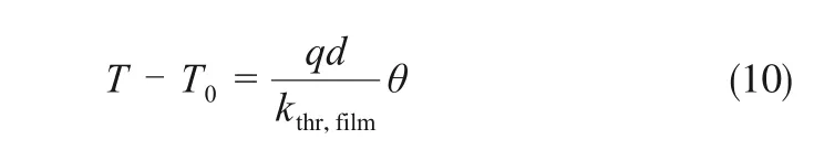
which linearly depends on the heat flux, i.e. the applied power.

1.2 Sensitivity analysis

The primary concern of the presented study is to figure out the correlation between sensitivity of T with respect to thermal parameters and the experimental conditions. The sensitivity of thermal parameters is intended to characterize the response of temperature distribution to the change of these parameters.In other words, the sensitivity of thermal parameters is the impact factors of these parameters on temperature distribution. Accordingly, the higher sensitivity of thermal parameters is desirable since it means the higher resolution of the MTPS for these thermal parameters. Therefore, the correlation between the sensitivity of thermal parameters and the experimental conditions can be utilized to identify how the experimental conditions determine the resolution of the MTPS method. For a thermal parameter η, its sensitivity coefficient STηis defined as

where the first-order differential is replaced by the first-order finite difference in numerical analysis,

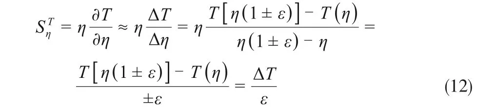
T (η) and T [η (1+ε )] correspond to a reference case and a case where only the parameter η under examination is varied by an amount of ε, respectively.On the experimental side, a meaningful analysis is possible only when the absolute ΔT is larger than the precision of thermocouples,say 0.1 K.

A dimensionless sensitivity coefficientreads

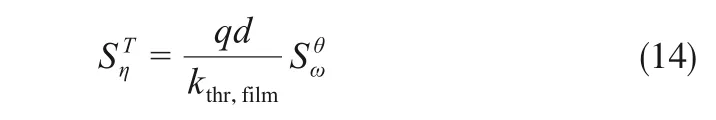
Considering the relation between T and θ,andare correlated via,

2 Results and discussion

In what follows, we are to employ the dimensionless model to evaluate how experimental conditions such as the heating protocol(flux and duration),the placement of thermocouples, and the geometry of samples affect the estimation precision of the MTPS method.

2.1 Heat flux

2.2 Placement of thermocouples

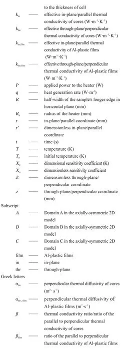
The placement of thermocouples on the sample surface has a major effect on identification of thermal parameters. In Figure 2, the sensitivity of four dimensionless thermal parameters φ,κ,β and Bi versus dimensionless time Fo is shown for the case with the parameters as listed in Table 2. The location of thermocouples varies from r=0 to 105 mm with a step of 10 mm.

Regarding φ, the sensitivity profiles first diverge and then converge into a single sloping line. On the contrary, the sensitivity profiles of κ, β and Bi are remarkably different during the whole period for different thermocouple locations. Quite interestingly,the sensitivity of κ, β and Bi levels off after a certain period of time. This difference lies in that κ, β and Bi are relevant to the heat conduction process while φ is relevant to the heat accumulation process. At the initial stage the temperature field is expanding due to 2D heat conduction, thus, the sensitivity profiles vary significantly.After the equilibrium of heat conduction,the temperature still increases linearly whereas the heat flux distribution is stationary. Therefore, the sensitivities of thermal parameters associated with heat conduction (κ, β and Bi) remain constant, while that of the thermal parameter (φ) associated with heat accumulation grows linearly.

Also of note,sensitivity profiles of β and Bi show transition between positive and negative values when r changes from 0 to 105 mm. This phenomenon is an inherent feature of 2D heat conduction process.As an immediate consequence, there must exist a special location at which point the sensitivity is 0, meaning that the temperature at this location is insensitive to thermal parameters.A word of caution is necessary to avoid these points in the selection of temperature monitoring locations.

The sensitivity magnitude of Bi is smaller than those of the other three. This difference is due to the fact that the influencing region of Bi is restricted to the interface between the core and the Al-plastic film,while those of the other three cover the whole core. In this model, we have introduced a thermal conductance λ to describe the thermal contact between the core and the film.λ,though being significant,has little effect on the temperature distribution as known from our previous work[5]. Hence, Bi and λ cannot be reliably identified from the presented method.

As the sensitivity magnitude of φ keeps increasing at the same rate after the initial stage, the placement of thermocouples has little effect on it. On the contrary, the placement of thermocouples has a pronounced effect on the identification of κ and β.As to κ, the sensitivity analysis suggests that thermocouples should be located as close as possible to the center of the heater.However,such placement is not always good for β, which matters more since it

Fig.2 Dimensionless sensitivity of four dimensionless thermal parameters((a)-(d)for φ,κ,β and Bi,respectively)versus di‐mensionless time Fo. The thermocouple locations vary from r’=0～0.95 with the step of 0.095.The red and the green lines are the threshold for dimensionless sensitivity magnitude when the applied power is 20 W and 80 W,respectively.characterizes anisotropic heat conduction in the core of LIBs.

Table 2 Model parameters for analysis on the effect of thermocouple placement

It is known from Eq. (14), given a specific heating power, the sensitivity magnitude should exceed a threshold to ensure that the absolute temperature difference ΔT is larger than the precision of thermocouples. In Fig. 6 (c), the green and red dotted lines denote the threshold for β when the applied power is 20 W and 80 W, respectively. This threshold lines defines the forbidden region of thermocouple placement, for example, 0.48＜r′＜0.67 is the forbidden region for 20 W. This forbidden region could be narrowed by intensifying the applied power.

2.3 Heating duration

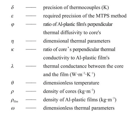
Once the heat flux and placement of thermocouples are determined, the next step is to determine the heating duration. A duration of 200 s was used in the previous work[5]. A more general principle for determining the heating duration is proposed here. The sensitivity of β at the location of(0, 0), named as the sensitivity of β at the pivot for convenience, is selected to evaluate the effect of the heat duration. Given the model input parameters as listed in Table 2, β is varied by adjusting kin, and the sensitivity is calculated then,as shown in Figure 3.

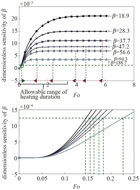
Fig.3 The sensitivity of β at the pivot at various levels of β.The green dotted line represents the threshold line for the case P=20 W.The intersection of this threshold line with the sensitivity profiles gives out the minimal heating duration.The red line gives out the maximal heating duration

At greater β, the initial stage in which the sensitivity ramps up is shortened. This phenomenon is attributed to the fact that the temperature difference in the horizontal plane vanishes quickly with a greater β.The green dotted line represents the threshold line for the case P=20 W. The intersection of this threshold line with the sensitivity profiles gives out the minimal heating duration. In other words, these intersection points define the lower bound of the heating duration.There is also an upper bound of the heating duration to ensure the axisymmetric temperature distribution.Therefore,the heating duration yields

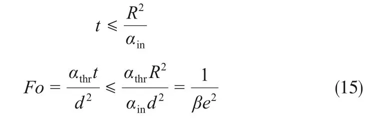
According to Eq. (15), the maximum heating duration increase with decrease in thermal conductivity ratio β and thickness-thickness ratio e.Therefore, the allowable range of the heating duration can be reduced at greater β.

The heating duration should be chosen between the lower bound in green and upper bound in red, as shown in Figure 3. Note that the sensitivity magnitude reflects the importance of the collected temperature data at corresponding time to parameter recognition.The monitored temperature data at various periods can be given various weighting scales according to the sensitivity magnitude. The data before the lower bound should weight on the lowest scale. The data at the time which exceeds the lower bound should weight on higher scale when the corresponding sensitivity is higher.

Besides the theoretical upper bound, a practical upper bound of the heating duration is considered to ensure the adiabatic boundary, to avoid disfunction of devices used in the experiment, and to prevent possible thermal hazard of LIBs.

2.4 Sample structure

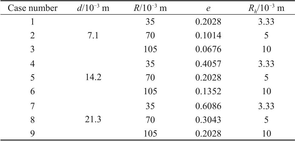
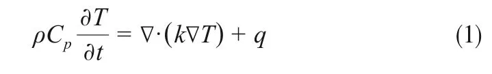
Table 3 Nine cases for evaluation of the structural effects

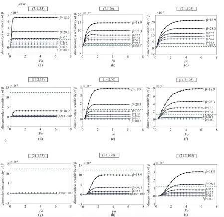
Fig.4 The sensitivity of β at the pivot at several levels of β corresponding to the selected cases with different combinations of(d,R).The dotted green line represents the threshold for the case of an applied power of 20 W.The case whose sensitivity profile transcends the threshold line is applicable to the MTPS method

3 Conclusions

This study investigated how experimental conditions affect the precision of the MTPS method.The precision of thermocouples defines a threshold,severing as the criterion for sensitivity analysis. The precision of the MTPS method is positively correlated with the power of the circular heater, which should be high but still under a threshold value defined by the safety criterion. There is an unfavorable region where thermocouples should not be arranged. This region is narrowed down by increasing the applied power. The lower bound of the heating duration increases at greater ratio of the parallel to perpendicular thermal conductivity. There is also an upper bound of the heating duration to ensure the axisymmetric temperature distribution. The MTPS method enjoys a much wider applicability of thermal conductivity ratio β for the LIBs with lower thickness-width ratio.Specifically, LIBs with the thickness-width ratio e larger than ～0.41 are suitable for the MTPS method,given c=0.1 and an applied power of 20 W. For LIBs beyond the application scope of the MTPS method, a thinner surrogate with the same mas1s ratio of each component and manufacture process as those of the original cell are required. Methodologically, the derived dimensionless solution and sensitivity is flexible to other methods of thermal parameter estimation.