XIE Xuezhi(谢学智)，GU Weizhe(谷伟哲)

(School of Mathematics，Tianjin University，Tianjin 300350，China)

Abstract: In the recent past few years，tensor，as the extension of the matrix，is well studied.Among many tensor related problems，the tensor complementarity problem(TCP)is a useful area for many researchers to study，and many methods to solve TCP have been proposed.In this article，under the condition of a strong P-tensor，we propose a smoothing Newton method to solve TCP based on the modulus-based reformulation，and we prove that the smoothing Newton method is globally convergent.Some numerical examples are given to demonstrate the efficiency of the smoothing Newton algorithm.

Key words: Tensor complementarity problem; Smoothing Newton method; Modulusbased reformulation

1.Introduction

The classical complementarity problem is to find a vector x ∈Rnsuch that

where F :Rn→Rnis a function and q ∈Rn.If F =Ax is a linear function where A ∈Rn×n，then (1.1) becomes

which is called a linear complementarity problem，denoted by LCP(A，q).[1]If F is a nonlinear mapping，then (1.1) is called a nonlinear complementarity problem，denoted by NCP.[2-4]In this paper，we consider F(x)=A xm-1，where A ∈R[m，n]is a tensor，and A xm-1is a vector defined by

with R[m，n]being the set of all real m-th order n-dimensional tensor.In this case，(1.1)becomes a special NCP such that

which is called a tensor complementarity problem，denoted by TCP(A，q).TCP as a generalization of LCP and NCP was firstly introduced by SONG and QI in[5]，and get further studied in[6-10]，such as XIE，LI and XU[8]proposed an iterative method to solve a lower-dimensional tensor complementarity problem.Because of the good properties of structural tensors，many algorithms for solving the tensor complementarity problem are obtained in recent years.

Recently，LIU，LI and VONG[11]proposed a nonsmooth Newton method to solve TCP based on a modulus-based reformulation.Before this，many good algorithms about modulusbased have been established for LCP.On the one hand，BAI[12-14]proposed a modulus-based matrix splitting and multisplitting iteration method for solving LCP，and presented convergence analysis for the established methods.Based on the splitting of system matrix A，the LCP is transformed into an implicit fixed-point equation，and a kind of matrix splitting iterative method based on module is established to solve large sparse LCPs.[15]On the other hand，[16] proposed a modulus-based nonsmooth Newton’s method for solving LCP.With the help of the methods for LCP，in this paper we pnopose a smoothing Newton method to solve the TCP based on a strong P-tensor.Firstly，we choose the strong P-tensor because a tensor complementarity problem has the property of global uniqueness and solvability (GUS-property)if and only if the tensor involved in the concerned problem is a strong P-tensor.[10]Then the smoothing Newton method has been widely used in NCP.[4，17-18]In order to use this method to solve the problem，we define a smooth approximation function.Under the above conditions of nonsingular，this method is well defined.It can be suitable for tensor complementarity problem based on the modulus-based reformulation and obtain good convergence.

The rest of this paper is organized as follows.In Section 2，we give some notations，definitions and preliminary results which are useful in the sequent analysis.In Section 3，under some sufficient conditions，we establish a smoothing Newton method to solve the TCP based on the modulus-based reformulation，and show the convergence of the method.In Section 4，we give some numerical examples to show the efficiency of the proposed algorithm.Conclusions are given in Section 5.

2.Preliminaries

In this section，we give some necessary notations，and review five definitions and four propositions，which will be used in the sequent analysis.

In this paper，for any differentiable function F : Rn→R，F′(x) denotes the Jacobian matrix of mapping F at x.The norm ‖·‖ denotes the Euclidean norm.For two matrices A = (aij)，B = (bij) ∈Rm×n，we write A ≥B(A ＞B) iffaij≥bij(aij＞bij) holds for all 1 ≤i ≤m and 1 ≤j ≤n，and denote

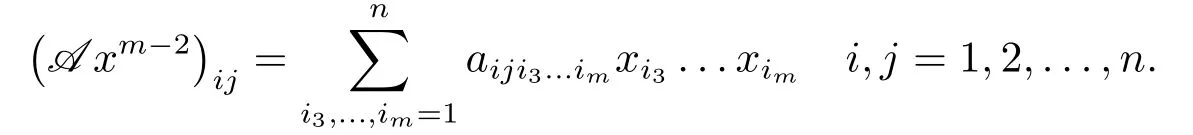
A m-order n-dimensional tensor is denoted by A = (ai1i2···im)1≤i1，...im≤n.Denote the set of all real m-th order n-dimensional tensor by R[m，n].Compare with A xm-1∈Rn，and A xm-2∈Rn×ncan be expressed as

When m = 2，R[m，n]is the set of all real matrices of n×n，which is usually denoted by Rn×n.For any A = (ai1i2···im) ∈R[m，n]is called a symmetric tensor，iffthe entries ai1i2···imare invariant under any permutation of their indices.Denote the set of all real m-th order n-dimensional symmetric tensor by S[m，n].For any A = (ai1i2···im) ∈R[m，n]，the diagonal entry of A is ai1i2···imwith i1= i2= ··· = im; others are called off-diagonal entries.A is called a diagonal tensor，iffall its off-diagonal entries are zero (we use I to denote the unit tensor，which is a diagonal tensor with each diagonal entry being 1).In particular，I represents the unit matrix.

Then，we give some definitions and propositions of the strong P(P0)-tensor.

Definition 2.1[19]A tensor A ∈R[m，n]is said to be a strong P(P0)-tensor，iffA xm-1+q is a P(P0)-function.

Definition 2.2[19]A mapping F : S ⊆Rn→Rnis said to be P(P0) function on S，if＞(≥)0 for all x，y ∈S with xy.

Definition 2.3[19]A matrix M ∈Rn×nis said to be a P(P0) matrix，ifffor each x ∈Rn{0}，there exists an index i ∈[n] such that x0 and xi(Mx)i＞(≥)0.

Proposition 2.1[19]Let A ∈S[m，n]，A xm-1+q is a P(P0)-function，iffits Jacobian matrix is a P(P0)-matrix.

Proposition 2.2[20]If A ∈Rn×nis a P-matrix，B ∈Rn×nis a positive diagonal matrix with 0 ＜B ＜I，then I-B+AB is a P-matrix.

Proposition 2.3[10]Suppose that A ∈R[m，n]is a strong P(P0)-tensor，then TCP(A，q)(1.2) has the GUS-property.

The following theorem detects the relationship between a modulus-based equation and the TCP(A，q)(1.2).The proof can be obtained from [11].

Theorem 2.1[11]A vector |x|+x ∈Rnis a solution of the TCP(A，q)(1.2) if and only if the vector x ∈Rnis a solution of the following system of equations:

where |x|=(|x1|，|x2|，··· ，|xn|)T∈Rn.

Thus，to search the solution of TCP(A，q)(1.2) can be equivalent solving the modulusbased equation (2.1).In [11]，LIU proposed a nonsmooth Newton method to the modulusbased equation (2.1).In this paper，we use a smooth Newton method to solve the modulusbased equation (2.1) with a smooth approximation function.Here is the definition.

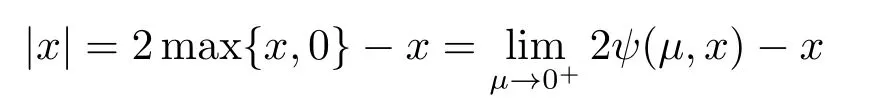
Definition 2.4It is well-known that

From the equation，we can see |x|=2 max{x，0}-x.We define a function ψ(µ，x):R2→R satisfying max{x，0}=The function is as follow:

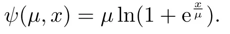
The function ψ(µ，x) is infinitely differentiable function of x，which is a smooth function on R.So we define

Definition 2.5Through Definition 2.4，in order to solve the equation in Rn，we define Ψ :Rn+1→Rnby

where µ＞0，x ∈Rn.

From the above definitions，to solve the equation

is equivalent to solve the equation

where the function f(µ，x):Rn+1→Rnis defined by

Proposition 2.4(i) We introduce a merit function H(x)=f(µ，x)‖2.When µ is a sufficient small positive number，we have that H(x) = 0 at x is equivalent to f(µ，x) = 0 at x.

(ii) Since f(µ，x) is continuously differentiable at x with µ＞0，and its Jacobian matrix

It is obvious that x is a solution of f(µ，x) = 0 ⇔x is a solution of the modulus-based equation F(x)=x-|x|+A(|x|+x)m-1+q =0 ⇔|x|+x is a solution of TCP(A，q)(1.2).Next，the main work is to solve f(µ，x) = 0.Since the function f(µ，x) is continuously differentiable for any x ∈Rnwith µ＞0，we can apply a smoothing Newton method to solve the system of smooth equations f(µ，x) = 0 at each iteration and let µ be a sufficient small positive number.So the solution of the problem(2.1)can be found.The smoothing Newton’s method is a classic method for solving the nonlinear equation G(x)=0 with

where G:Rn→Rnis a continuously differentiable function.This is the fundamental idea of the algorithm.In the next section，we will introduce the algorithm in detail.

3.A Smoothing Newton Algorithm

In this section，in order to solve the equation (2.1) we apply a smoothing Newton algorithm to solve the f(µ，x) = 0.Without affecting the final experimental results，we fix µ to a sufficient small positive number，and we use the following assumption to ensure that the algorithm is well-defined and globally convergent.

Assumption 3.1Assume A ∈R[m，n]is a strong P tensor，q ∈Rn，and the function A xm-1+q is a P function.

Remark 3.1If the function A xm-1+ q is a P function，then the corresponding(m-1)A xm-2is a P matrix，which is a good condition for the smoothing Newton algorithm.

Now，we give the algorithmic framework.

Algorithm 3.1(A Modulus-Based Smoothing Newton Algorithm)

Step 0 Choose σ ∈(0，1).µ＞0 is a sufficient small positive number，and x0∈Rn.Set k :=0.

Step 1 If H(xk)=0，stop.Otherwise，go to Step 2.

Step 2 Compute Δxk∈Rnby

Step 3 Let ikbe the minimum of the values 0，1，2，··· such that

Step 4 Set xk+1:=xk+2-ikΔxkand k :=k+1.Go to Step 1.

Under the assumptions，we discuss Algorithm 3.1 is well defined and analyze the convergence of Algorithm 3.1.Firstly we discuss Algorithm 3.1 is well-defined.

Proposition 3.1If the tensor A ∈R[m，n]is a strong P-tensor，the matrix(µ，x)obtained from above is nonsingular.

ProofSuppose that A ∈R[m，n]is a strong P-tensor，from Definition 2.1 and Proposition 2.1，we know that 2(m-1)A(2Ψ(µ，x))m-2(µ，x) is a P-matrix.Letting J(µ，x) =A(2Ψ(µ，x))m-2，from Definition 2.3，we know that there exists an index i ∈[n] such that x0 and xi(J(µ，x)(µ，x)x)i＞0.

Notice that the diagonal matrixµ，x) (see (2.4)) with µ＞0 satisfies

Lemma 3.1[17]Under the condition of Assumption 3.1 and µ＞0，for any {xk}，when‖xk‖→∞，we have

Lemma 3.2[17]Under the condition of Assumption 3.1，the infinite sequence {xk}generated by Algorithm 3.1，the sequences {H(xk)} is monotonically decreasing and

Lastly，we are in a position to show the convergence of Algorithm 3.1.

Theorem 3.1Suppose that Lemmas 3.1-3.2 and Assumption 3.1 are satisfied.Any accumulation point of {xk} generated by Algorithm 3.1 is a solution of H(x)=0.

ProofBy Lemma 3.2 ，the sequence {H(xk)} is monotonically decreasing，hence it is bounded.With the coercive property of H(x) in Lemma 3.1，the sequence {xk} must be bounded.Thus，the sequence{xk}has a convergent subsequence which we write without loss of generality as {}.Let x*be the limiting point of the sequence.By Lemma 3.2，we obtain that H(x*)=0.Then x*is a solution of the equation (2.1).This completes the proof.

4.Numerical Examples

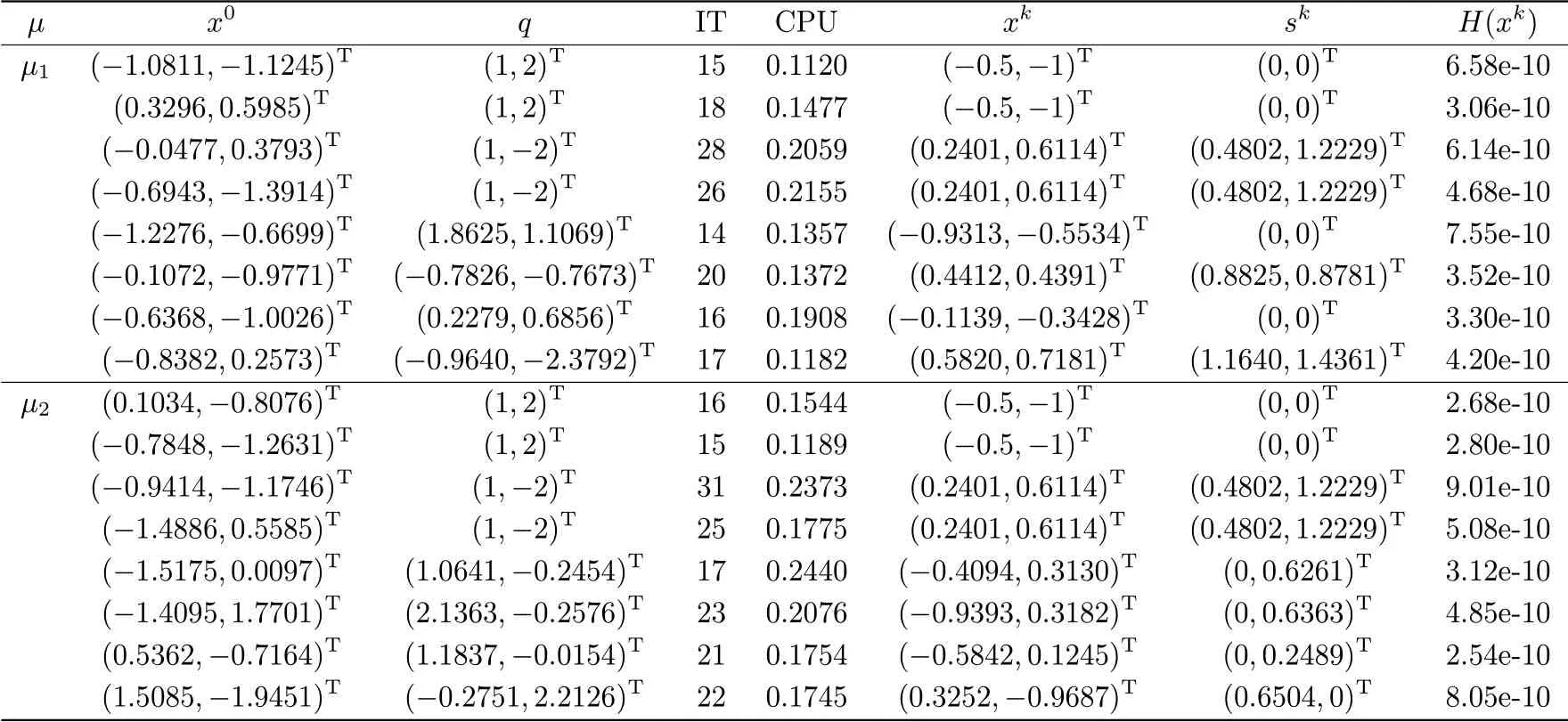
In this section，we give the numerical experiments to operate Algorithm 3.1.Firstly，we introduce some notations in the following tables.IT denotes the number of iterations，CPU denotes the running time(in seconds) required to complete the iteration process，x0denotes the initiation point of the algorithm，xkdenotes the points satisfying termination conditions，and sk(sk=|xk|+xk) is the approximate solution to the TCP(A，q)(1.2).The parameters used in the algorithm are chosen as σ =0.3.And we choose H(xk)≤10-9as the terminated the condition.

After observing the modulus-based equation (2.1)，we decide to choose different µ and randomly generated initial vector x0，q to test the algorithm，and choose Example 3.10 and Example 3.30 in [11] as the system tensor.

Example 4.1Firstly，within the calculation range allowed by Matlab，we takeµ1=0.01 and µ2= 0.005 as smooth parameters respectively，fix the A ∈R[3，2](see Example 3.30 in[11]) with a111= a222= a121= a221= 1，a122= a211= -1，and other entries are zeros，and choose randomly generated initial vector x0，q.

After our experiment of Example 4.1，we get eight pieces of data withµ=0.01.From the first four data，we can see the solutions are same as Tab.4 in [11].As for the last four data，the algorithm can get different solutions in an acceptable accuracy with randomly generated q and x0.We also make µ = 0.005，and the results are same as µ = 0.01.All the numerical results are shown in the Tab.4.1.

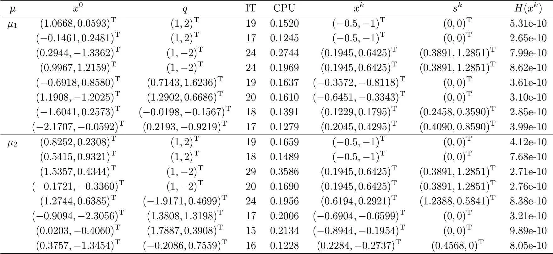
Tab.4.1 Numerical results for Example 4.1 with µ1 =0.01 and µ2 =0.005

Example 4.2In this example we choose the system tensor A ∈R[4，2](see Example 3.10 in [11]) with a1111=a2222=a1122=a2211=1，a1222=a2111=-1，and other entries are zeros.µ1and µ2are same as Example 4.1.x0and q are randomly generated.

In Example 4.2，we can see the condition is same as Example 4.1，and no matter how we choose the initial value，the algorithm works well in an acceptable accuracy.The results are shown in Tab.4.2.

In this section，all tests of the examples were done in Matlab R2014b and Tensor Toolbox 2.6.The codes were done on a DELL desktop with Inter(R) Core(TM) i5-5200U CPU 2.20 GHz and 4GB RAM running on Windows 7 system.After the tests for the smoothing Newton algorithm 3.1 with different parameter µ，randomly generated initial points x0and q，we can see that Algorithm 3.1 is efficient and stable，and the solution xkcan solve the equation(2.1).From Theorem 2.1，|xk|+xkis a solution of the TCP(A，q) (1.2).

Tab.4.2 Numerical results for Example 4.2 with µ1 =0.01 and µ2 =0.005

5.Conclusion

In this article，we proposed a smoothing Newton method for solving the TCP(A，q)(1.2)，and convert the TCP(A，q)(1.2) to the modulus-based equation (2.1).LIU，LI and VONG[7]proposed a nonsmooth Newton method to solve the modulus-based equation (2.1).Now we define a smooth approximation function and propose a smoothing Newton method to solve the modulus-based equation(2.1).Then we test some examples for Algorithm 3.1，and the results showed the algorithm is efficient.However，it is well-known that many people reformulate the modulus-based equation as an implicit fixed-point equation and use the fixed point iterative algorithms to solve the equation in [8-9].But no one has established the fixed point iterative algorithms for the modulus-based equation (2.1) with tensor.So this is our work to do in the future.