S.Kshrisagar,A.Francis,J.J.Yee,S.Natarajan and C.K.Lee

Abstract:In this paper,the node based smoothed-strain Abaqus user element (UEL)in the framework of finite element method is introduced.The basic idea behind of the node based smoothed finite element (NSFEM)is that finite element cells are divided into subcells and subcells construct the smoothing domain associated with each node of a finite element cell [Liu,Dai and Nguyen-Thoi (2007)].Therefore,the numerical integration is globally performed over smoothing domains.It is demonstrated that the proposed UEL retains all the advantages of the NSFEM,i.e.,upper bound solution,overly soft stiffness and free from locking in compressible and nearly-incompressible media.In this work,the constant strain triangular (CST)elements are used to construct node based smoothing domains,since any complex two dimensional domains can be discretized using CST elements.This additional challenge is successfully addressed in this paper.The efficacy and robustness of the proposed work is obtained by several benchmark problems in both linear and nonlinear elasticity.The developed UEL and the associated files can be downloaded from https：//github.com/nsundar/NSFEM.

Keywords:Smoothed finite element method (SFEM),node based SFEM (NSFEM),linear and nonlinear elasticity,Abaqus UEL (user elements),compressible and nearlyincompressible materials.

1 Introduction

The classical FEM is a well established numerical method for simulation of real world problems related to science and engineering.The commercial finite element software like Abaqus is widely used in such applications.The Finite Element Analysis (FEA)involves three steps viz.pre-processing,analysis and post-processing.The pre-processing stage focuses on discretization of problem domain into non-overlapping sub-domains known as finite elements.This process of discretization is known as meshing.In classical FEM,shapes of the elements are restricted to triangles and quadrilaterals in two dimensions and tetrahedra and hexahedra in three dimensions [Altair Hypermesh Documentation (2014)].

Due to these restrictions on element topology,the accuracy of the classical FEM is highly influenced by mesh distortion [Lee and Bathe (1993)].In this regard,the triangular elements are considered to be robust for meshing but not in terms of accuracy like quadrilateral elements [Chandrupatla and Belegundu (2016)].Therefore,a lot of time is spent in generation of well conditioned quadrilateral elements.The present work is restricted to two dimensional problems discretized with triangular elements;however,the solution accuracy is comparable to the quadrilateral elements.This is possible by using SFEM proposed by Liu et al.[Liu,Dai and Nguyen-Thoi (2007)].Various methods proposed in the SFEM framework are the Cell Based SFEM (CSFEM),Node Based SFEM (NSFEM),Edge Based SFEM (ESFEM),Face Based SFEM (FSFEM),Selective SFEM,α-FEM,β-FEM and other variations [Zeng and Liu (2016)].All the SFEM methods are applicable to triangular,quadrilateral or polygonal elements.These methods are well established with characteristics like convergence properties,stability,accuracy,and computational complexity [Nguyen-Xuan,Bordas and Nguyen-Dang (2008)].Also the methods can be easily extended to three dimensional and geometric nonlinearity with nearly-incompressible material problems [Lee (2016)].Kumbhar et al.[Kumbhar,Francis,Swaminathan et al.(2018);Wang (2014)],developed UEL to implement the CSFEM over the Polygonal Finite Element Method (PFEM)and the classical FEM in the commercial software Abaqus.Using CSFEM on two dimensional problems discretized with triangular elements,provides the numerical results exactly same as the classical FEM [Liu,Dai and Nguyen-Thoi (2007)].The NSFEM is found to be suitable to work with triangular elements and less sensitive to mesh distortion and locking issues [Liu,Nguyen-Thoi,Nguyen-Xuan et al.(2009)].

In this work,Abaqus UEL is developed for the NSFEM and confined to the two dimensional problems.However this work can be easily extended to three dimensional problems.The problem domain is completely discretized using Constant Strain Triangular(CST)elements.The CST elements are chosen because the commercial software available can discretize any complex two dimensional geometry using CST elements without much difficulty [Altair Hypermesh Documentation (2014)].Also the use of CST elements ease the construction of node based smoothing domain.Since,for the triangular elements,each node in the domain is associated with the one-third area of the corresponding attached element.All such regions for each node are known as smoothing regions.Therefore,the Abaqus UEL for NSFEM requires nodal coordinates and element connectivity of all the CST elements attached to each node under consideration.This data is provided to the Abaqus UEL through external data file.Depending upon the number of attached CST elements,the Abaqus UEL definition changes.For this purpose,a master UEL is written which incorporates different UEL elements defined as subroutines.The two dimensional linear and nonlinear elasticity problems are solved taking into account nearlyincompressible materials.For nonlinear large strain problems,hyperelastic material model,the quasi-compressible neo-Hookean model in this work,is used.The complete paper is divided in the following sections：the governing equations for the elasticity problems,NSFEM Abaqus implementation section explains the procedure involved for the NSFEM framework,the numerical examples section that validates the developed UEL by solving few benchmark problems and followed by the conclusion section.

2 Smoothed finite element approximation

In this section the governing equations are first presented for two dimensional linear elasticity and then its Smoothed finite element approximation is derived.In the subsequent subsection,the equations pertaining to weak form of two dimensional nonlinear elasticity accounting geometric nonlinearity are presented.The neo-Hookean hyperelastic material model and the Newton-Raphson iterative method equations for obtaining nonlinear solution are presented in brief.

2.1 Smoothed finite element approximation in linear elasticity

Let us consider a two dimensional isotropic linear elastic body in d ({≡1,2 })dimensional Euclidean space,ℝd,whose material point is given byx=∑xIeI,whereeIare the vectors of a chosen basis.LetΩ⊂ℝdrepresent the body with domain boundaryΓ.The body with domain boundaryΓ≡δΩconsisting of Dirichlet boundaryΓuand Neumann boundaryΓt,such thatΓ=Γu∪ΓtandΓu∩Γt= Ø and the outward normal toΓisn.Given the body forceb,the Cauchy stress tensorσ,the prescribed displacementand the tractiont̅,to find the displacement fielduthe governing differential is written as below：

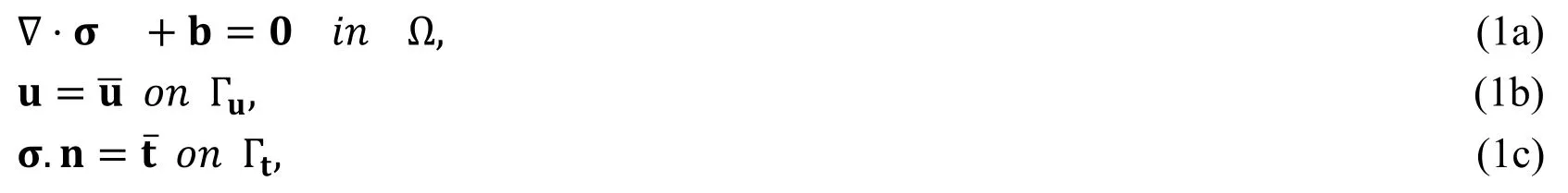
LetU(Ω)={u:Ω→ℝd|uI∈H1(Ω),I=1,...,d,u=uonΓu} be the displacement trial function andV(Ω)={v:Ω→ℝd|vI∈H1(Ω),I=1,...,d,v=0onΓu} be the test function spaces,whereH1denotes the Hilbert-Sobolev first order space.The variational form of Eq.(1a)is written as below：

The Cauchy stress tensorσand strain tensorεcan be expressed as：

where shear modulusμand Lamé’s first parameterλcan be expressed by Young’s modulusEand Poisson’s ratiovas follows：

The strain tensorεis given as：

Note that,since the relation of the Cauchy stress tensor and strain tensor is given asσ=Dε,the material modulus matrixDcan be defined as：

In the following,it is assumed that the arbitrary domain is partitioned intonelfinite elements defined assuch thatΩ≡and∩= Ø,∀I≠J.For the discretization of the weak form,let the setU(Ω)⊂H1consist of polynomial interpolation functions of the following form：

whereφedenote the finite element shape functions.Substituting these displacement functions in Eq.(2),the corresponding weak form can be obtained as：

Using the arbitrariness of testing displacement functionvℎ,this can be reduced to the following form：

In Eq.(9),Kis the global stiffness matrix andB=∇φis the strain-displacement matrix that is computed using the derivatives of the shape functionsφfor each element in case of the classical FEM.Liu et al.[Liu,Dai and Nguyen-Thoi (2007a)] employed SFEM converting area integration to line integration through the divergence theorem while performing numerical integration.The basic idea of SFEM is to divide the problem domain into sub-domains where strains are smoothed.These strains are constant over the smoothing domains but they are discontinuous across the boundaries of these smoothing domains.The smoothing domains are constructed using the topology provided by the mesh.For a single CST element shown in Fig.1(a),NSFEM smoothing domains for respective nodes are marked with distinct features.

Figure1:NSFEM smoothing domains for a CST element

The smoothed strain-displacement matrixBIfor nodeIis evaluated as below：

whereAIis the area of the smoothing domain,nis the outward normal vector andΨIis the shape functions.Referring to Fig.1(b),it is observed that overall numerical integration consists of line integration over the smoothing domain boundaries in SFEM compare to classical FEM.Such a line integration is evaluated using the shape function value at one Gauss point located at mid-point of the line boundary and the corresponding outward normal.After the evaluation of the strain-displacement matrix,construction of global stiffness matrixKis similar to classical FEM.Thus in SFEM numerical integration is dependent on node coordinates in physical space avoiding locking and element distortion issues associated with classical FEM.The detailed construction and simplified evaluation of the strain displacement matrix for NSFEM having more than one CST elements will be explained in Section 3.1.

2.2 Smoothed finite element approximation in finite elasticity.

Here for the completeness of the subsection,few important equations and outline of the nonlinear elasticity solution is presented.However the elaborate derivations and detailed discussions of nonlinear elasticity accounting geometric nonlinearity and nearly incompressible material are found in Bhat [Bhatti (2006)].

Galerkin variational form for finite elasticity can be written as：

whereWis the strain energy density.

In this work,the compressible neo-Hookean model is used [Bhatti (2006)]：

where the right Cauchy-Green tensorCand the JacobianJare defined asC=FTFandJ=detFrespectively.The deformation gradientFcan be evaluated as：

whereXis the initial configuration andxis the current configuration expressed asx=X+u.

Note that,the left hand side and the right hand side of the Eq.(11)are defined as internal forces and external forces respectively：

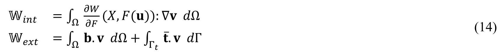
The Newton-Raphson iterative method is used for the estimation of nonlinear solution.In this method,initial solution is assumed as zero and a residual is generated in Eq.(11).Subsequent incremental solutions are estimated using directional derivative ofWintandWext.The equation for residualRuwith the current displacement functionucan be written as：

To estimate incremental iterative displacementΔu,Eq.(13)can be expressed with the directional derivative ofWintandWextas follows：

where the directional derivative for work done by internal forcesDΔuWintis given as：

wherei,j,k,l∈(1,2)for two-dimensions.Note thatDΔuWext=0 as external forces will be unaffected by displacement changes except external pressure forces which are deformation dependent.

Combining Eq.(16)and Eq.(17)gives a system of linear equations.Solution of this system of linear equations leads to the estimation of displacement incrementΔu.With the new displacementuiter+1=uiter+Δuiter,residualRuis recalculated.To get more accurate solutions,the residual is required to be minimum.

3 NSFEM Abaqus implementation

3.1 Construction of node based smoothing domain in the framework of Abaqus UEL definition

Fig.2 shows an example of the construction of node-based smoothing domainΩc.As shown in Fig.2,when node c is selected as the target node,neighboring CST elements are divided into subcells by mid-points and centroids.Each neighbored subcell with vertices labelled,e.g.,a1,c,a11 and a12,is connected to anti-clockwise manner.When connected subcells make a closed region,it is called as the smoothing domain.The straindisplacement matrixBNRof the smoothing domainΩccan be evaluated as follows [Liu,Nguyen-Thoi,Nguyen-Xuan et al.(2009)]：

whereANRis the area of the smoothing domainΩc,Nis the number of CST elements sharing node c,Anis the area of CST element andBnis the strain-displacement matrix of CST element in FEM.Since the compatible strain is constant in CST element,simplified node-based strain-displacement matrixBNR(Eq.(20))can be used in the proposed Abaqus UEL.

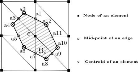
Figure2:Node-based smoothing domain associated with a target node

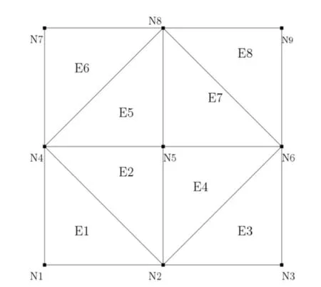
Figure3:Discretization of a square domain by triangular meshes with nodes labelled N1 to N8 and elements labelled E1 to E8

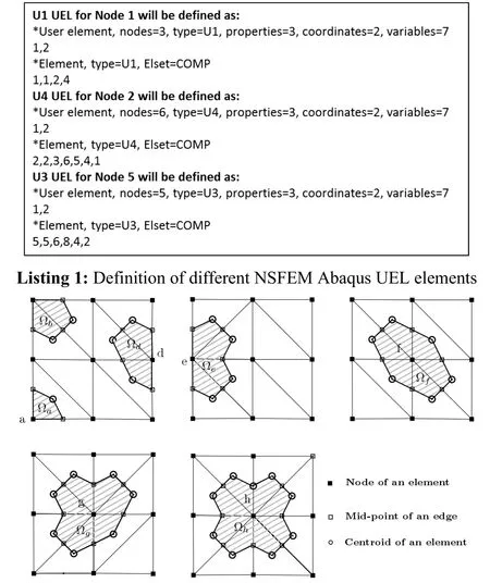
Figure4:Smoothing domains for the NSFEM Abaqus UEL elements U1 to U7

For the NSFEM Abaqus UEL definition,first let discretize a square domain with triangular meshes as shown in Fig.3.Then it needs to be found element cells associated with each node,for example,Node N1 is contained to node vertices of element E1 while node N2 is attached to elements E1 to E4.This means that targeted node N1 is attached to only element E1 and node vertices of element E1 are N1,N2 and N4.Similarly,for node N2,attached elements have node vertices N1,N2,N3,N4,N5 and N6.This node information for the proposed UEL definition is given in Listing 1,sampling node N1,N2 and N5 with prefix N dropped.The different NSFEM UEL element numbering like U1,U2,U3,etc.is used according to the number of nodes of attached elements.The number of variables in the UEL is chosen according to analysis requirements.It can be also observed in Listing 1 that the number of nodes in the NSFEM Abaqus UEL is equal to UEL specific number after letter U plus two.In addition,similar property Abaqus UEL elements can be grouped together and can be given a particular name for easy reference.In the same manner,different definition types of smoothing domains corresponding to the NSFEM Abaqus UEL are given in Fig.4.

3.2 Major steps in the NSFEM Abaqus UEL implementation

Fig.5 depicts the three major steps involved in the implementation of the NSFEM Abaqus UEL：1)Pre-processing,2)Analysis using NSFEM Abaqus UEL and 3)Post-processing.

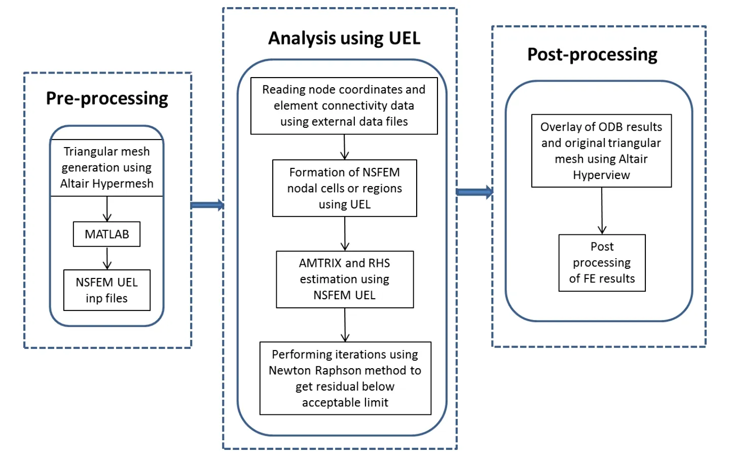
Figure5:Major steps involved in the implementation of NSFEM Abaqus UEL

3.2.1 Pre-processing

The first stage of the proposed UEL element is the pre-processing where the problem domain is discretized using CST elements.For the domain discretization,the mesh generation software Altair Hypermesh [Altair Hypermesh Documentation (2014)] is used.NSFEM Abaqus UEL is defined using the nodes of attached elements as explained in the previous section.A MATLAB code is used to obtain node vertices of elements associated with the considering node.Once the attached elements are found,their node vertices are arranged after the target node to define NSFEM Abaqus UEL.Data set of node coordinates and node connectivity of CST elements is used as input parameters for the MATLAB code.The data files of the NSFEM Abaqus UEL definition are automatically generated using the MATLAB code.

Before proceeding towards the analysis stage,input data file compatible with the developed UEL requires to share the following common Keywords [Abaqus Documentation (2012)]：*user element to define the UEL and *UEL property to define thickness and material properties for element groups.In the keyword of *user element,the NSFEM Abaqus UEL elements labelled like U1,U2,U3,etc.need to be matched appropriately with the corresponding element type in the Abaqus input data file.Moreover,the NSFEM Abaqus UEL elements having the same number of nodes can be grouped into one and given a specific name.Rest of the structure of input data file is similar to the typical Abaqus standard input data file.

3.2.2 Analysis using SFEM Abaqus UEL

The next stage is to run the analysis using NSFEM Abaqus UEL.For the analysis Abaqus standard solver can be invoked by the following command：

abaqus job=＜inp file name＞ user=＜fortran Abaqus UEL file name＞ other options

This command is much similar to the one used for other types of Abaqus UEL.The difference with NSFEM Abaqus UEL is that the data file containing the data set of CST element node coordinates and node connectivity is provided during the analysis.Such data file is kept in the same file path as the other analysis files.Note that,this data file path and its name need to be carefully mentioned in the definition of the NSFEM master UEL.In this stage use of the NSFEM Abaqus UEL FORTRAN code for the analysis is included as well.

3.2.3 Post-processing

Once the analysis is completed,Abaqus output data base (ODB)file containing the requested result is generated in the last stage.Since Abaqus CAE does not support postprocessing of Abaqus UEL elements without significant modifications,Altair Hyperview[Altair Hypermesh documentation (2014)],in the present work,is used for the postprocessing.In this case Abaqus ODB results file and Abaqus input data file containing CST elements are overlaid for the post-processing.

3.2.4 The details of the NSFEM Abaqus UEL FORTRAN code

To complete the implementation of the NSFEM,following FORTRAN code for Abaqus UEL is required.In this work,the NSFEM Abaqus UEL structure is arranged as a master UEL which further calls an individual UEL like U1,U2,etc.as a subroutine.The outline of the master UEL is shown in Listing 2.The master UEL starts with the name of the subroutine with the list of arguments in the parentheses.Parameters section includes names of the constants which are assigned a fixed value.This leads the identification of constants easy while using them in the FORTRAN code.RHS and AMATRIX matrices denote the residual force and stiffness contribution of each element respectively are also completely defined in the UEL.Additional variables such as numnode,numelem,node and element are added in the UEL to read node coordinates and elements connectivity data from an external data file as shown in Listing 2.

The structure of the data file contains total number of nodes at the top and followed by node coordinates.It is ensured that all the nodes are renumbered.Using the node numbers,their coordinates are arranged in ascending order.In this work,node numbers can be eliminated as sequence itself dictates the node number.If the renumbering of nodes is not done,it is necessary to include the node numbers in the data file.After the node coordinates in the data file,total number of CST elements in the domain are written and this is followed by node connectivity data of the CST elements.Similar to the node renumbering,the same comments are applied to the element renumbering.The if statement in the NSFEM master UEL is used to select the corresponding UEL subroutine according to the NSFEM Abaqus UEL element type.

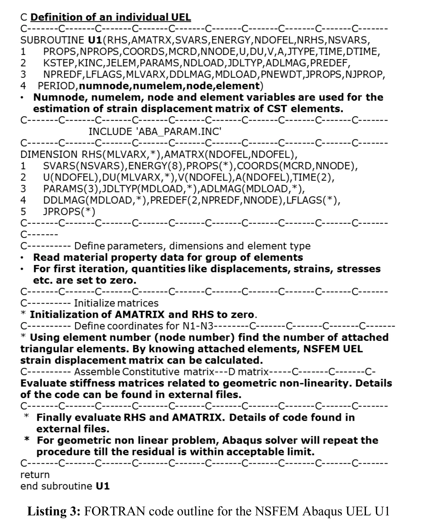
A detailed definition of a UEL U1 is shown in Listing 3.In this detailed code,it can be observed that element number of NSFEM Abaqus UEL which is actually the node for which the smoothing domain is defined.This node number is used for finding the attached CST elements.Eq.(20)is used for the calculation of thestrain-displacement matrix constructed over the NSFEM smoothing domain.The detailed subroutine definition helps in the estimation of RHS and AMATRIX of the corresponding NSFEM smoothing domain.The estimation of global stiffness matrix by assembling of the matrices of individual UEL elements is taken care by Abaqus.

The Newton-Raphson iterative method is used for correcting the nonlinear stiffness of the model in the same manner with the conventional FEM.Abaqus handles the iterative method once the linear and nonlinear stiffness matrices are defined correctly in the NSFEM Abaqus UEL subroutine.Material properties are read by the keyword *UEL property from the Abaqus input data file.Iterations are performed till it satisfies the convergence criteria as set in the Abaqus analysis parameters.Overall the major difference in the analysis using NSFEM Abaqus UEL is the estimation of the node-based strain-displacement matrix over smoothing domains but the rest of the process is the same as FEM4All MATLAB and FORTRAN codes are downloadable and available on Github(hppts：//github.com/nsundar/NSFEM).

4 Numerical examples

In this section,a series of numerical examples is solved to demonstrate the utility of Abaqus NSFEM UEL elements：a cantilever beam,a bevelled cantilever beam,a square plate with a hole and a sharp V-notched square plate.For the tests,two dimensional linear elasticity reference problem is taken from Liu et al.[Liu,Dai and Nguyen-Thoi(2007)] and nonlinear elasticity considering geometric nonlinearity with nearlyincompressible material reference problems is chosen from Lee [Lee (2016)].Obtained numerical results are compared with Abaqus results with quadrilateral elements.

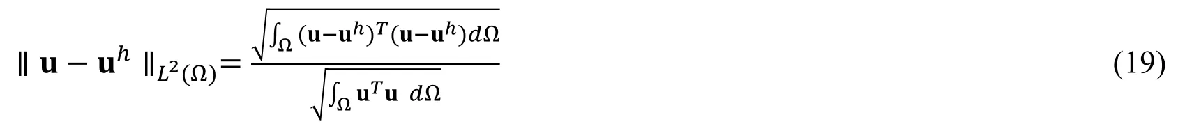
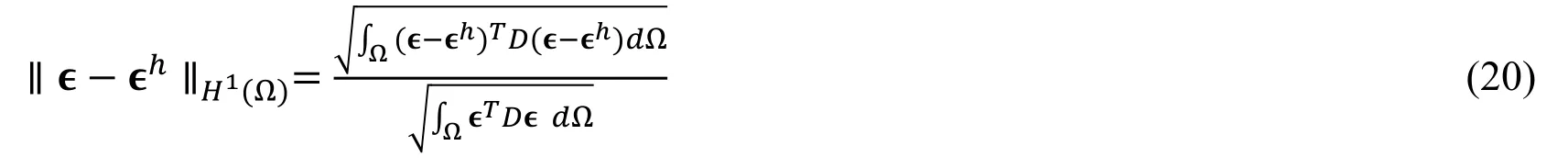
The accuracy and the convergence rate using different Abaqus elements are analyzed using the relative error norm in the displacement and strain energy as given by：

Displacement norm：

Strain energy norm：

4.1 Patch test

In this section,two patch tests are performed on arbitrary patches of elements to satisfy basic convergence requirements of rigid body displacements and constant strain conditions to validate Abaqus NSFEM UEL.Note that,the material properties are Young’s modulusE=1000.0 Pa and Poisson’s ratiov=0.3 and only pre-described displacement boundary conditions are considered for the tests.

Firstly,a rigid body motion displacement is considered with an arbitrary patch of CST elements as shown in Fig.6(a).The pre-described horizontal displacements which is 1.0 m are imposed on boundary nodes a1,a2,a3,a4,a7,a9 and a10.In this test,as a result,the computed horizontal displacements at interior nodes a5,a6 and a8 should be 1.0 m.As shown in Fig.6(b),obtained results show that Abaqus NSFEM UEL passes the test.

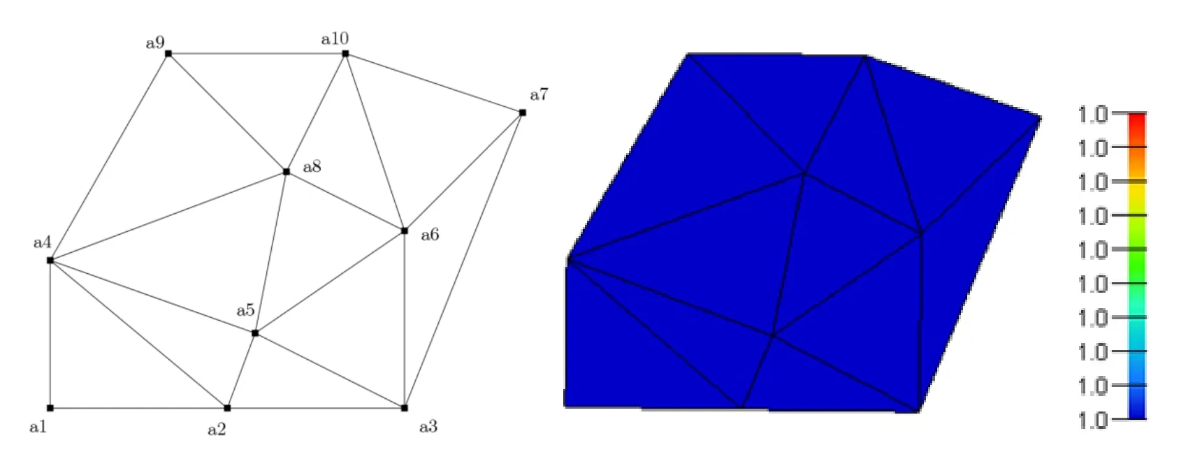
Figure6:Rigid body motion displacement test with CST elements：(a)geometry of the patch and (b)constant strain displacement results

In the next test,linear displacementsu=xare imposed on the boundary nodes b1,b2,b3,b4,b6,b7,b8 and b9 for the patch as shown in Fig.7(a).In order to pass this constant strain patch test,interior node b5 must show horizontal displacement equal to itsxcoordinate.As shown in Fig.7(b),Abaqus NSFEM UEL also passes the constant strain displacement test.

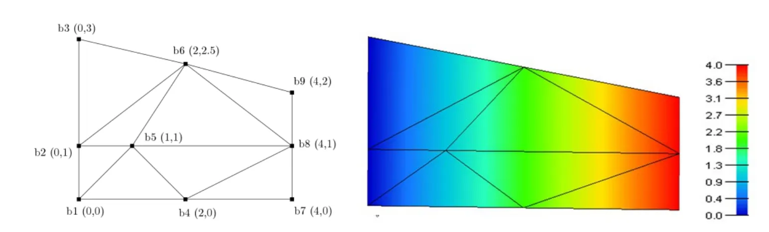
Figure7:Constant strain displacement test with CST elements：(a)geometry of the patch and (b)constant strain displacement results

4.2 Cantilever beam in linear elasticity

The geometry of a cantilever beam with lengthL=48.0 m and widthD=12.0 m and CST element discretization are shown in Fig.8.The material parameters for the plate areE=3.0×107Pa,v=0.3 and the total parabolic shear load acting over the free edge isP=-1000 N.

The exact analytical solution for the above problem is given by：

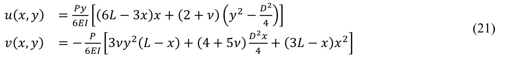
whereI=D3/12 is the moment of inertia and a state of plane stress is considered.

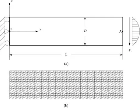
Figure8:The geometry of a cantilever beam：(a)geometry and boundary conditions and(b)discretization of the beam with CST elements

The convergence rates of the relative error in displacement norm and strain energy norm are given in Fig.9.It is clearly seen that Abaqus NSFEM UEL shows better results than that using Abaqus triangular elements without any change in the domain discretization.These results are encouraging in the sense that analysis with NSFEM Abaqus UEL elements provide comparable results as those obtained using Abaqus quadrilateral elements with the same solver.In the next subsections,two dimensional nonlinear elasticity problems are considered.

4.3 Cantilever beam in geometric nonlinearity

In this section,the geometric nonlinearity is investigated.For this test,the cantilever beam used in the previous section is considered again.The parabolic shear load 10,000 N is implemented on the right-end edge and the left-end edge of the beam is completely constrained in all DOFs.The reference solution for this test is obtained by Abaqus with the very fine meshes (526,850 DOFs).

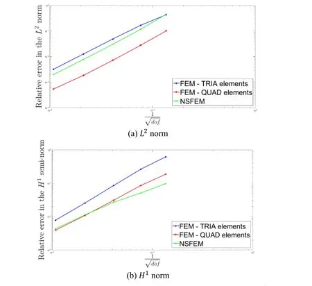
Figure9:The convergence of the relative error for the cantilever beam：(a)L2 norm and(b)H1 semi-norm

Fig.10 illustrates the deformed shapes of the beam for Abaqus QUAD CPS4I and the proposed Abaqus NSFEM UEL elements and an improved accuracy obtained by the proposed elements can be observed in Tab.1.

TheL2error norm convergence rate for this test is shown in Fig.11.NSFEM UEL elements result shows better convergence rate than triangular elements and it is comparable to quadrilateral elements as shown in Fig.11.

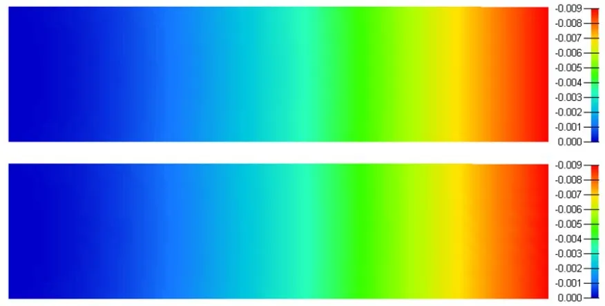
Figure10:Deformed shapes of the cantilever beam with the vertical displacement plot：(a)Abaqus QUAD CPS4I and (b)Abaqus NSFE UEL elements

Table1:The vertical displacements at the sampling point ‘A’ of the cantilever beam Reference solution：-0.08907 (m)

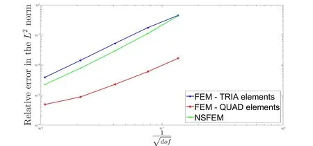
Figure11:The convergence of the relative error in the L2 norm for the cantilever beam

4.4 Bevelled Cantilever beam

A bevelled cantilever beam is studied in this section for the quasi-incompressible hyperelasticity.The geometry of the beam is given in Fig.12 withL1=0.5 m and vertical loadP1=-0.1 N/m.In this work,the neo-Hookean model is used with shear modulusμ=0.6 Pa and bulk modulusk=107Pa equivalent to Poisson’s ratiov=0.49999997.Abaqus with very fine meshes (526,338 DOFs)is also used as the reference solution for this problem.

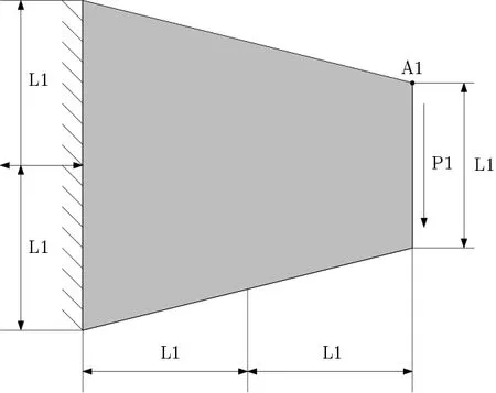
Figure12:The geometry of a bevelled cantilever beam

The deformed shapes of the bevelled beam for Abaquas CPE4I and Abaqus NSFEM UEL elements are shown in Fig.13 and their detailed displacement values at the sampling point ‘A1’ are given in Tab.2.The results solved using NSFEM Abaqus UEL are in agreement with the results provided in Lee [Lee (2016)].

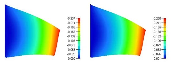
Figure13:Deformed shapes of the bevelled cantilever beam：(a)Abaqus quadrilateral CPE4I and (b)Abaqus NSFEM UEL elements

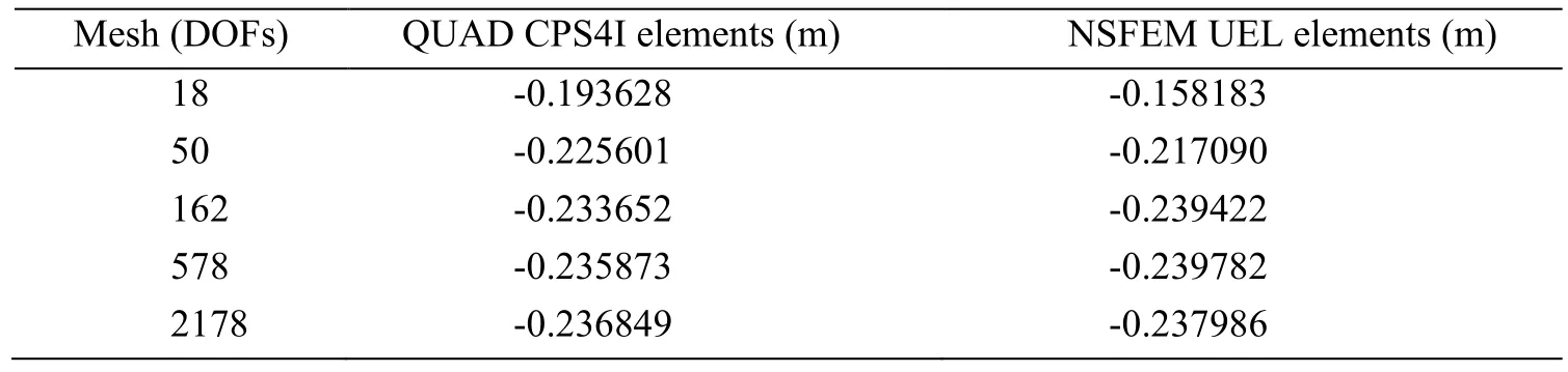
Table2:The vertical displacements at the sampling point ‘A1’ of the bevelled beam

The convergence of theL2error norm is depicted in Fig.14.It is observed from Fig.14 that Abaqus NSFEM UEL provides better convergence rate than Abaqus triangular element.In addition the following displacement and convergence results are confirmed again：the proposed Abaqus UEL is comparable to fully integrated elements.

Figure14:The convergence of the relative error in the L2 norm for the bevelled cantilever beam

4.5 A square plate with a hole

In this section,nonlinear nearly-incompressible problem is once again demonstrated.The problem domain is given as a square plate with a hole at the center (see Fig.15).

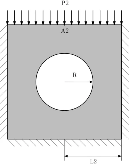
Figure15:The geometry of a square plate with a hole at the center

The geometry of the plate isL2=1.0 m and the radius of the circle is given asR=0.5 m.Vertical external forceP2=-0.1 N is equally distributed on the top edge of the plate.The neo-Hookean material with Lamé’s parametersμ=1.8 Pa andk=107Pa are used (Poisson’s ratiov=0.49999997).Right,left and bottom edges are fully constrained in all DOFs.The reference solution to the square plate with a hole problem is obtained using Abaqus with fine CPE4I element meshes having 791,712 DOFs.Fig.16 shows deformed shapes of the square plate for Abaqus quadrilateral and the proposed NSFEM UEL elements.A comparison of vertical displacements of Abaqus CPE4I and Abaqus NSFEM UEL elements is given in Tab.3 with detailed values.The results of vertical displacement obtained at the sample point ‘A2’ show an upper bound solution using NSFEM Abaqus UEL elements while that Abaqus CPE4I elements give a lower bound solution.

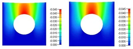
Figure16:The deformed shapes of the plate：(a)Abaqus quadrilateral CPE4I and (b)the proposed Abaqus NSFEM UEL

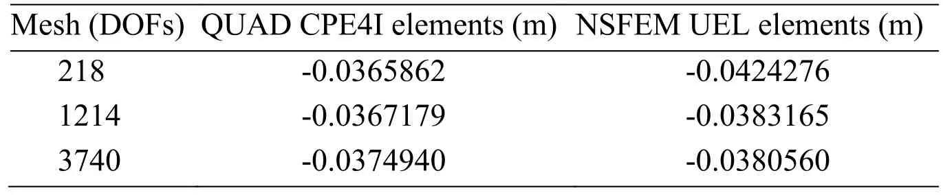
Table3:The vertical displacements at the sampling point ‘A2’ of the square plate Reference solution：-0.0349782 (m)

4.6 A sharp V-notched square plate

Lastly,a square plate with a sharp V-notch is studied.The geometry of the plate is given asL3=1.0 m andB=0.02 m as shown in Fig.17.The loading parameter is given as the total vertical loadP3=0.05 N on the top edge and shear modulusμ=0.6 Pa and bulk modulusk=105Pa are used (v=0.499997).The bottom edge of the plate is constrained in all DOFs and the vertical displacement results are reported at the point ‘A3’.

Figure17:The geometry of a square plate with a sharp V-notch

Abaqus CPE4I element with the fine meshes (526,850 DOFs)is used as the reference solution for this test.The deformed shapes of Abaqus CPE4I and Abaqus NSFEM UEL for the plate are illustrated in Fig.18.The detailed vertical displacements obtained at the sampling point ‘A3’ can be found in Tab.4.Similar to the previous plate with a hole problem,the proposed UEL elements provide the upper-bound solution whereas Abaqus CPE4I results lower-bound solution.

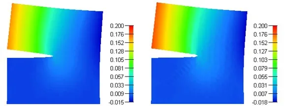
Figure18:The deformed shapes of the V-notched plate：(a)Abaqus quadrilateral CPE4I and (b)Abaqus NSFEM UEL elements

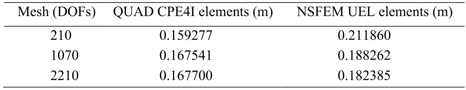
Table4:Sharp V-Notch square plate point ‘A3’ vertical displacement results summary Reference solution：0.16986 (m)

5 Conclusions

In this work,Abaqus NSFEM UEL is successfully implemented in Abaqus software for two dimensional linear and nonlinear problems.The following conclusions can be drawn based on the results presented：

1)The proposed Abaqus NSFEM UEL simplifies the preprocessing process as only CST elements are used.

2)The proposed Abaqus NSFEM UEL provides more accurate results compare to the conventional FEM results even when the problem domain is completely discretized with linear triangular elements.

3)This is improvisation in available FEM code.The convergence rate of Abaqus NSFEM UEL results are at par with those obtained from fully integrated Abaqus quadrilateral elements accounting additional complexities like geometric nonlinearity and nearly-incompressible material.

4)The proposed Abaqus NSFEM UEL provides upper bound solution while the conventional FEM provides lower bound solution.Combining these two methods,range bound solution for the problem under consideration can be easily predicted without any major changes.

Acknowledgement:J.J.Yee and C.K.Lee would like to thank the National Research Foundation (NRF)of Korea through Ministry of Education (No.2016R1A6A1A03012812)for providing financial support for this research undertaking.