Yan-Hong Yao(姚雁鸿) and Xin-He Meng(孟新河)

Department of Physics,Nankai University,Tianjin 300071,China

(Received May 1,2019)

AbstractIn this paper,we interpret the dark energy phenomenon as an averaged effect caused by small scale inhomogeneities of the universe with the use of the spatial averaged approach of Buchert.Two models are considered here,one of which assumes that the backreaction termand the averaged spatial Ricci scalar obey the scaling laws of the volume scale factorat adequately late times,and the other one adopts the ansatz that the backreaction termis a constant in the recent universe.Thanks to the effective geometry introduced by Larena et al.in their previous work,we confront these two backreaction models with latest type Ia supernova and Hubble parameter observations,coming out with the results that the constant backreaction model is slightly favoured over the other model and the best fitting backreaction term in the scaling backreaction model behaves almost like a constant.Also,the numerical results show that the constant backreaction model predicts a smaller expansion rate and decelerated expansion rate than the other model does at redshifts higher than about 1,and both backreaction terms begin to accelerate the universe at a redshift around 0.5.

Key words:cosmological model,dark energy,cosmological backreaction effect

1 Introduction

According to recent observations of type Ia supernovae,the universe is in a state of accelerated expansion.[1−2]The simplest scenario to account for these observations is a positive cosmological constant in Einstein’s equations(The most well known cosmology model including such constant is the so called Lambda cold dark matter(ΛCDM)model),which is assumed to be an effect of quantum vacuum fluctuations.However,because of the huge discrepancy between the theoretical expected value and the observed one,other alternative scenarios have been proposed,including scalar field models such as quintessence,[3]phantom,[4]dilatonic,[5]tachyon,[6]and quintom[7]etc. and modified gravity models such as braneworlds,[8]scalar-tensor gravity,[9]higher-order gravitational theories.[10−11]Since the so called fitting problem that how well is our universe described by a standard Friedmann-Lemaˆıtre-Robertson-Walker(FLRW)model is not solved yet,recently a third alternative has been considered to explain the dark energy phenomenon as an averaged effect caused by small scale inhomogeneities of the universe.[12−13]

In order to consider cosmology model without assuming an FLRW background,it is necessary to answer a longstanding question that how to average a general inhomogeneous model.To date the macroscopic gravity(MG)approach[14−17]is probably the most well known attempt at averaging in space-time.Although it is the only approach that gives a prescription for the correlation functions,which emerge in an averaging of the Einstein’s field equations,so far it required a number of assumptions about the correlation functions,which make the theory less convictive.Therefore,in this paper we adopt another averaged approach which is put forward by Buchert,[18−19]in despite of its foliation dependent nature,such approach is quite simple and hence becomes the most well studied theoretical framework of averaged models.Since the averaged field equations in such approach do not form a closed set,one needs to make some assumptions about the backreaction term appeared in the averaged equations.In Ref.[20],by taking the assumption that the backreaction termand the averaged spatial Ricci scalarobey the scaling laws of the volume scale factor,Buchert proposed a simple backreaction model.To confront such model with observations,Larena et al.presented the effective geometry with the introduction of a template metric that is only compatible with homogeneity and isotropy on large scales of FLRW cosmology instead of on all scales.[21]As was pointed out by Larena et al.,the scaling solution cannot be expected to fully represent the realistic backreaction effect throughout the whole history of the universe since we expect that the realistic backreaction term will change considerably at redshift10.However,since we only use the datasets of type Ia supernova and observational Hubble parameter in this paper,we merely concern the behavior of the backreaction term at adequately late times,i.e.,which means that although we assumeobeys scaling laws of aDin such redshift range,it can behave very differently at higher redshifts,particularly,such term encounters rapid change whenbecause of the structure formation effects,and becomes negligible whenwhich is reasonable because of the consistence between perturbation theory predictions and CMB observations.Nevertheless,we still doubt that the scaling solution is a prime description of the late-time backreaction term,so we propose another parameterization ofby simply setting it as a constant at late times,and it turns out that such model is preferred by observations.We use the natural units c=1 throughout the paper.

The paper is organized as follows.In Sec.2,the spatial averaged approach of Buchert is demonstrated with presentation of the averaged equations for the volume scale factor aD.In Sec.3,we introduce the template metric,which is a necessary tool to test the theoretical preditions with observations,and computation of observables.In Sec.4,we apply a simple likelihood analysis of two backreaction models by confronting them with latest type Ia supernova and Hubble parameter observations.After analysis of the results in Sec.5,we summarize our results in the last section.

2 The Backreaction Models

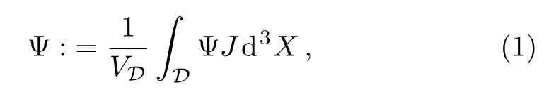
In Ref.[18],Buchert considered a universe filled with irrotational dust with energy density ϱ.By foliating spacetime with the use of Arnowitt-Deser-Misner(ADM)procedure and defining an averaging operator that acts on any spatial scalarfunction as

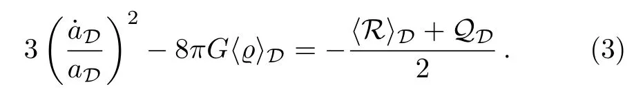
and the averaged Hamiltonian constraint

One can then obtain a specific backreaction model with an extra ansatz about the form ofA popular choice is to assume that

where n and p are real numbers,whileandrepresent the present value of the backreaction term and the averaged spatial Ricci scalar respectively.There are two types of solutions found in Ref.[20].The first type,with n=−2 and p=−6,is less important since at late times it corresponds to a quasi-Friedmannian model in which the backreaction effect can be neglected.The second type,which demands n=p,has the explicit expression as:

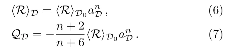
As mentioned above,we only assume such parameterization of the backreaction term to be valid in the recent universe.

By introducing the following dimensionless parameters:

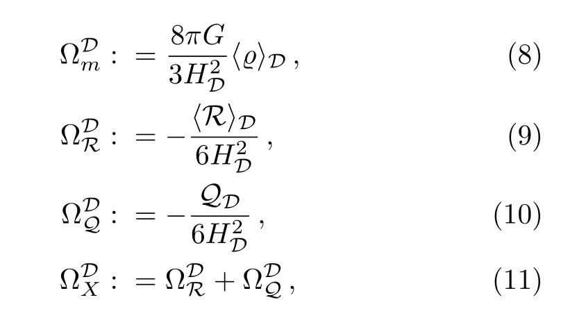
one can express the volume Hubble parameterand the volume deceleration parameteras:

In this paper,we propose another backreaction model with the assumption that the backreaction term is a constant at late times of the universe,which means,by using the integrability condition,QDand ⟨RDhave the following expression:

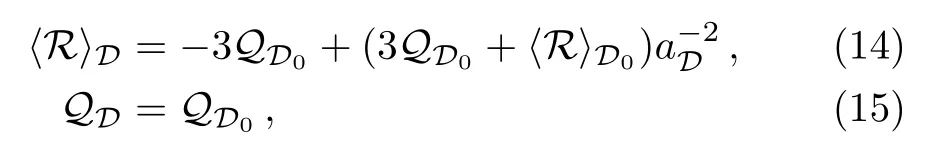
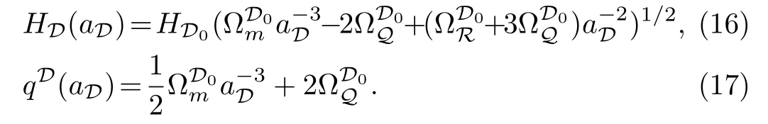
from which one can obtain the volume Hubble parameter HDand the volume deceleration parameter qDin this backreaction model as follow with the use of the averaged equations

3 Effective Geometry

3.1 The Template Metric

In Ref.[21],a template metric was proposed by Larena et al.as follows,

where LH0=1/HD0is the present size of the horizon introduced so that the coordinate distance is dimensionless,and the domain-dependent effective three-metric reads:

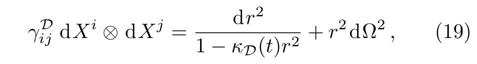
with dΩ2=dθ2+sin2(θ)dϕ2,this effective three-template metric is identical to the spatial part of an FLRW metric at any given time,but its scalar curvaturecan vary from time to time.As was pointed out by Larena et al.,cannot be arbitrary,more precisely,they argue that it should be related to the true averaged scalar curvaturein the way that

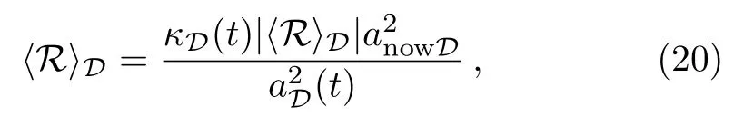
which is taken as one of the assumptions for two models considered in this paper.

3.2 Computation of Observables

The computation of effective distances along the light cone defined by the template metric is very different from that of distances in FLRW models.Firstly,let us introduce an effective redshiftdefined by

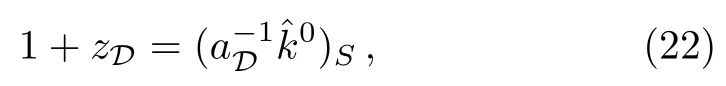
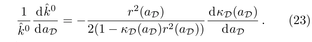
where the letters O and S denote the evaluation of the quantities at the observer and at the source respectively,gabin this expression represents the template metric,while uais the four-velocity of the dust,which sat is fiesuaua=−1,kathe wave vector of a light ray traveling from the source S towards the observer O with the restrictions kaka=0.Then,by normalizing this wave vector such that(kaua)O=−1 and introducing the scaled vector=,we have the following equation:

As usual,the coordinate distance can be derived from the equation of radial null geodesics:

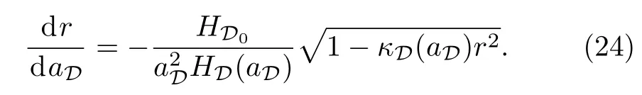
Solving these two equations with the initial condition(1)=1,r(1)=0 and then plugging(aD)into Eq.(22),one finds the relation between the redshift and the scale factor.With these results,we can determine the volume Hubble parameterand the luminosity distanceof the sources defined by the following formula

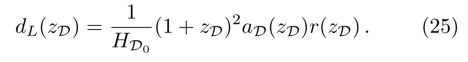
Having computed these two observables,it is then possible to compare the backreaction model predictions with type Ia supernova and Hubble parameter observations.

4 Constraints from Supernovae Data and OHD

In this section,we perform a simple likelihood analysis on the free parameters of two backreaction model mentioned above with the combination of datasets from type Ia supernova and Hubble parameter observations.

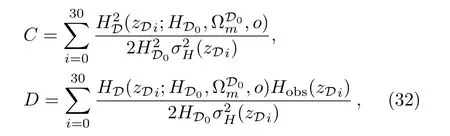
The best-fit values of the model parameters(Here o represents n in the case of scaling backreaction model andin the case of constant backreaction model respectively.)from the recently released Union2.1[22]compilation with 580 data points are determined by minimizing

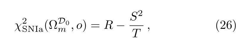
here R,S,and T are defined as

whereµobsrepresents the observed distance modulus and σµdenotes its statistical uncertainty.

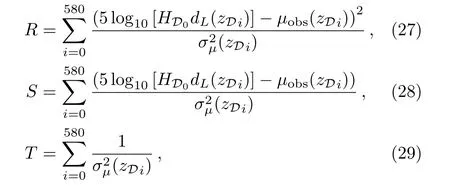
For the observed Hubble parameter dataset in Table 1,the best-fit values of the parameters(HD0)can be determined by a likelihood analysis based on the calculation of

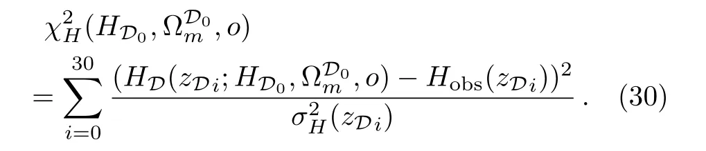
As Ma et al.[23]stated,the marginalized probability density function determined by integratingover HD0from x to y with a uniform prior reads

where

and

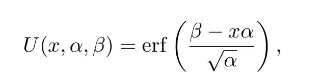
[x,y]is taken as[50,90],and erf represents the error function.

The fitting results attained from analyzingby using functions Findminimum and ContourPlot in mathematica are presented in Fig.1,Table 2 for the scaling backreaction model and Fig.2,Table 3 for the constant backreaction model.The comparison ofin these two tables show that the constant backreaction model is slightly favoured over the other model by current observations,confirming the correctness of our speculation that the scaling solution is not a prime description of the latetime backreaction term.Also,the result in Table 2 suggests that,the best fitting backreaction term in the scaling backreaction model behaves almost like a constant,which demonstrates the rationality to propose the constant backreaction model rather than other backreaction model in the beginning.Unlike the scaling backreaction model,according to Table 3 and Eq.(14),observations favor a monotone decrease averaged spatial Ricci scalar in the constant backreaction model,this dynamical behavior of the averaged spatial Ricci scalar reduces the best fitting value of the model parameter

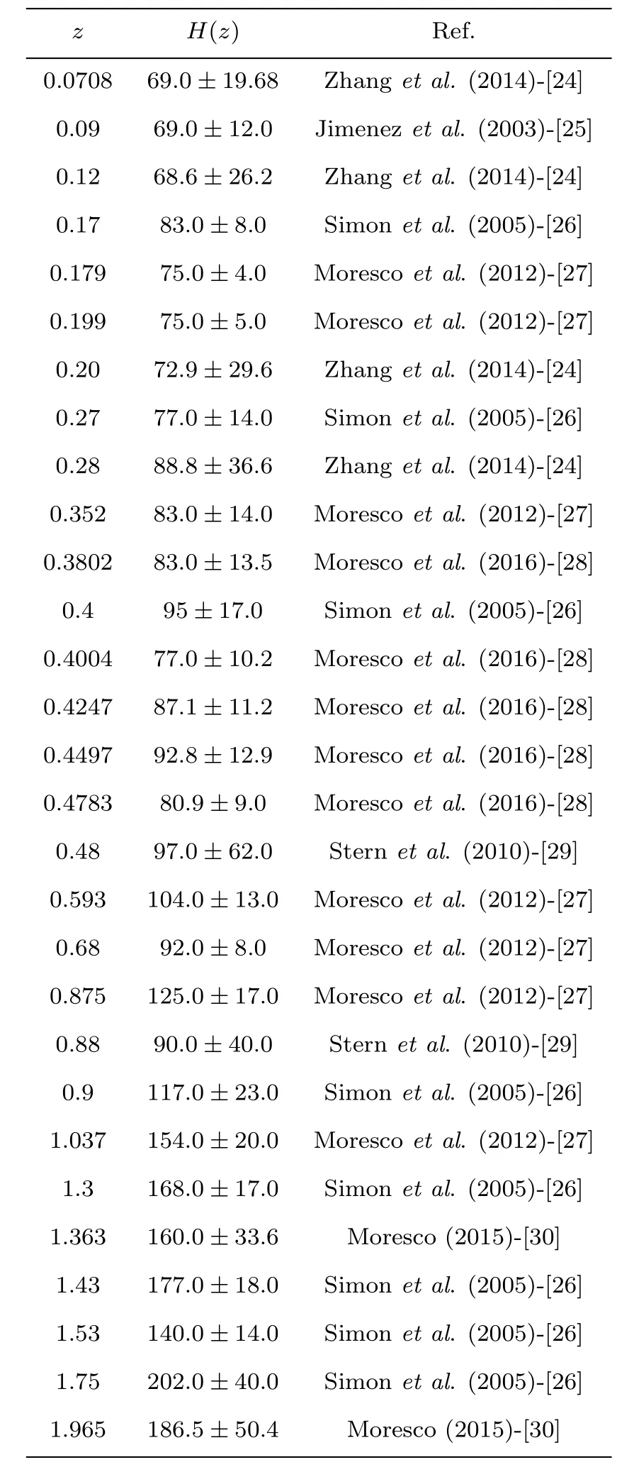
Table 1 The current available OHD dataset.

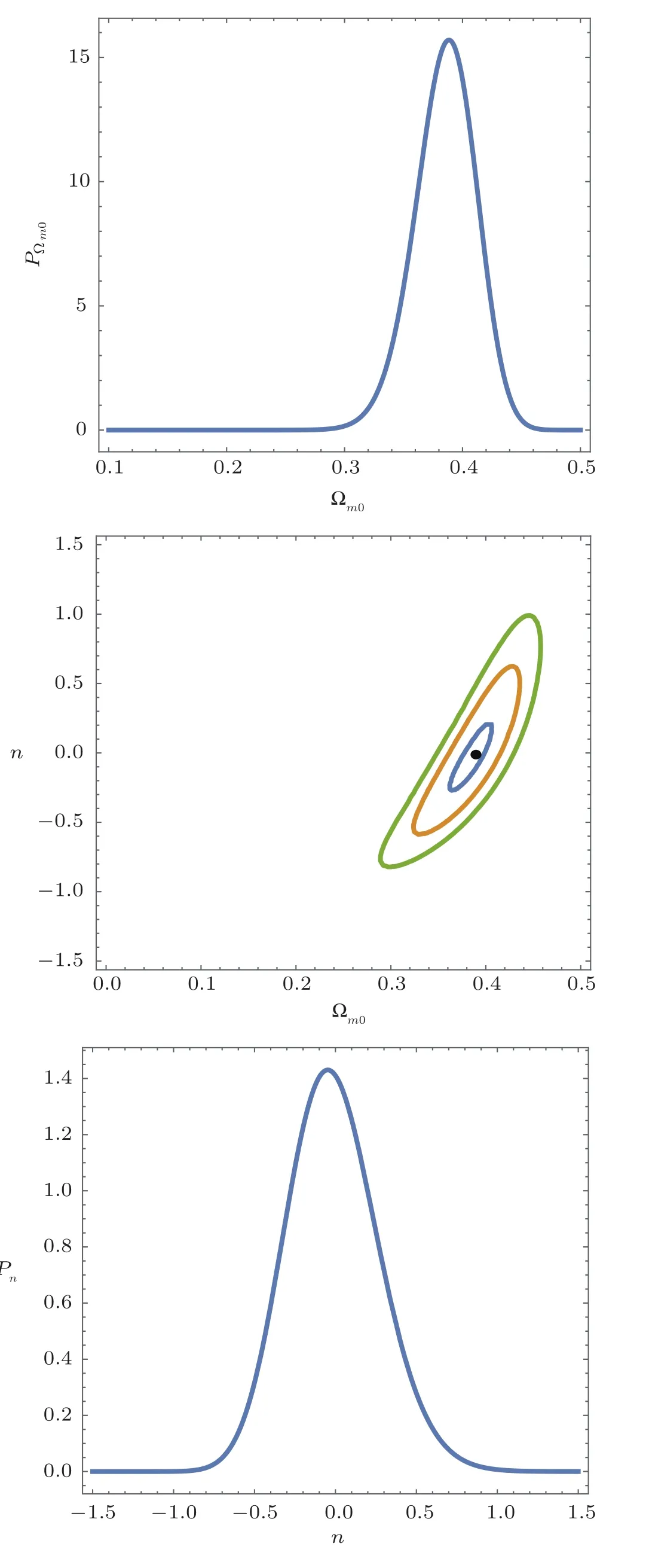
Fig.1(Color online)The 1σ,2σ and 3σ confidence regions and best fi tting point of of the free parameters,n for the scaling backreaction model,along with their own probability density function.The prior for∝H(0.5−)H(−0.1),The prior for n∝ H(1.5−n)H(n−(−1.5)),H(x)is the step function.

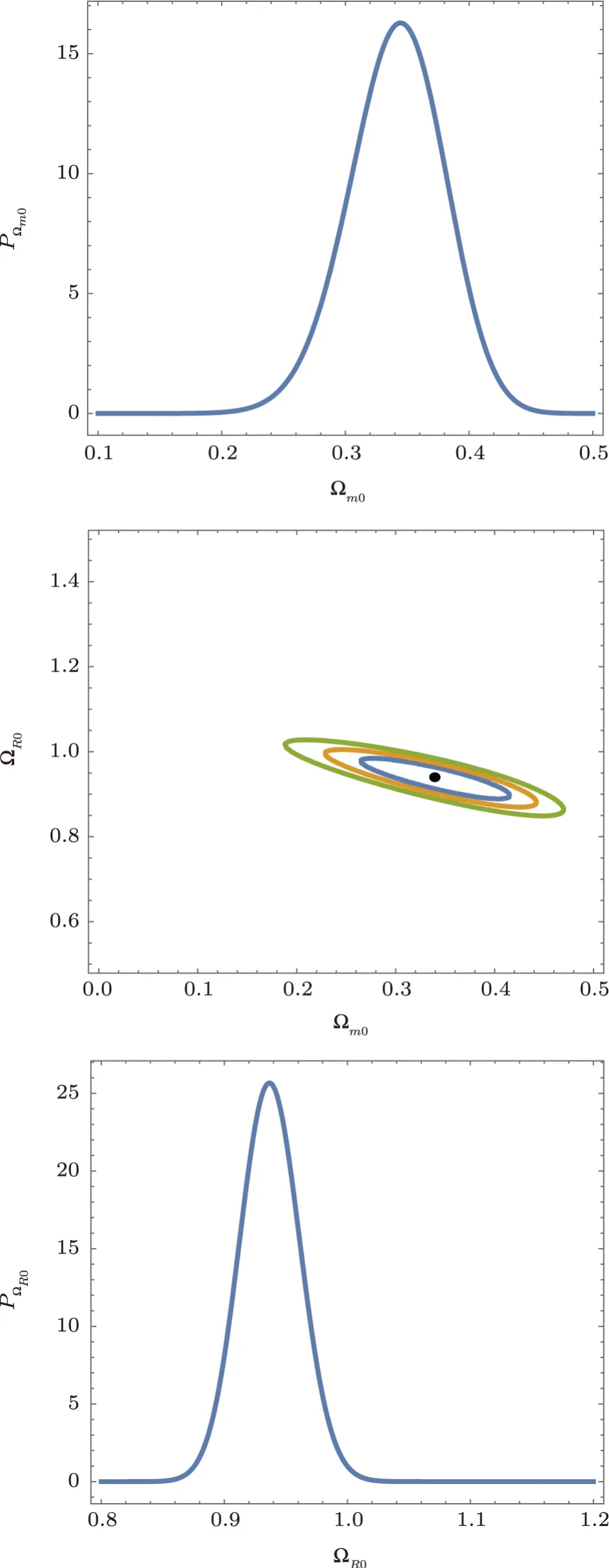
Fig.2 (Color online)The 1σ,2σ and 3σ con fi dence regions and best fitting point of the free parametersfor the constant backreaction model,along with their own probability density function. The prior for ∝,The prior for ∝ H(1.2−,H(x)is the step function.

Table 2 The fitting results of the parameters(,n)with 1σ region in the scaling backreaction model,is corresponding to(,n)=(0.39,−0.01).

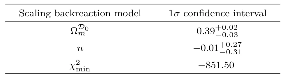
Table 2 The fitting results of the parameters(,n)with 1σ region in the scaling backreaction model,is corresponding to(,n)=(0.39,−0.01).

Scaling backreaction model 1σ confidence intervalΩD0 m 0.39+0.02−0.03 n −0.01+0.27−0.31 χ2min −851.50

Table 3 The fitting results of the parameters(,)with 1σ region in the constant backreaction model,is corresponding to()=(0.33,0.93).

Table 3 The fitting results of the parameters(,)with 1σ region in the constant backreaction model,is corresponding to()=(0.33,0.93).

Constant backreaction model 1σ confidence interva ΩD0 m 0.33+0.05−0.03ΩD0 R 0.93+0.03−0.03 χ2min −853.07

Fig.3(Color online)The evolution of HD/HD0and qD with respect to zD.Here the blue line and the orange line are corresponding to that of the scaling backraction model and the constant backreaction model with best-fit parameters.

Noting from the fitting results that the best-fit value of the matter density parameter in the scaling backreaction model is bigger than that in the other model,indicating that this model predicts a larger expansion rate and decelerated expansion rate at high redshifts.Such departure is shown in Fig.3,which also reveals that the universes described by two models with their best-fit parameters share the almost same expansion rate and decelerated expansion rate(accelerated expansion rate)oncedrops below about 1,and enter a stage of an accelerated expansion with a redshift around 0.5.

5 Conclusion and Discussion

In this paper,the dark energy phenomenon has been interpreted as an averaged effect caused by small scale inhomogeneities of the universe.In order to understand the averaged evolutional behavior of the universe within the approach of Buchert,we have considered two backreaction models,one of which assumes that the backreaction termand the averaged spatial Ricci scalarobey the scaling laws of the volume scale factorat adequately late times,and the other one adopts the ansatz thatis a constant in the recent universe.With the aid of the effective geometry introduced by Larena et al.in their previous work,we have confronted these two backreaction models with latest type Ia supernova and Hubble parameter observations,and found that the best fitting backreaction term in the scaling backreaction model behaves almost like a constant,which demonstrates the rationality to propose the constant backreaction model rather than other backreaction model in this paper.Moreover,as is shown by the results of numerical analysis,the constant backreaction model predicts a smaller expansion rate and decelerated expansion rate than the other model does at redshifts higher than about 1 and both backreaction terms begin to accelerate the universe at a redshift around 0.5.

Although we only make assumptions about the specific form of the backreaction term at late times throughout the paper,a complete backreaction model must consider the specific behavior of the backreaction term at arbitrary redshift.Nevertheless,parameterization of the late-time backreaction term is helpful and necessary for searching a complete backreaction model that is also favoured by observations at high redshifts.