Huanyao WEN(温焕尧) Lei YAO(姚磊) Changjiang ZHU(朱长江)†

1.School of Mathematics,South China University of Technology,Guangzhou 510641,China

2.School of Mathematics and Center for Nonlinear Studies,Northwest University,Xi’an 710127,China

E-mail:mahywen@scut.edu.cn;leiyao@nwu.edu.cn;machjzhu@scut.edu.cn

Abstract The two-phase flow models are commonly used in industrial applications,such as nuclear,power,chemical-process,oil-and-gas,cryogenics,bio-medical,micro-technology and so on.This is a survey paper on the study of compressible nonconservative two- fluid model,drift- flux model and viscous liquid-gas two-phase flow model.We give the research developments of these three two-phase flow models,respectively.In the last part,we give some open problems about the above models.

Key words compressible nonconservative two- fluid model;drift- flux model;viscous liquidgas two-phase flow model;well-posedness

1 Compressible Nonconservative Two- fluid Model

1.1 Research background-1

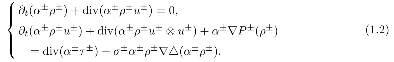
One of the typical two-phase flow models,called compressible nonconservative two- fluid model,is

The variable α+,α−∈ [0,1]are the volume fraction of liquid and gas,satisfy=1;are,respectively,the densities,the velocities and the pressures of each phase,and the two pressure functions satisfy,where A±>0,¯γ±>1 are constants,f(·)is a known smooth function,it can be a zero function(in this case,the two pressures are equal);are the viscous stress tensors,µ±and λ±are shear and bulk viscosity coefficients,satisfying µ±>0,2µ±+dλ±≥ 0;σ±are the capillary coefficients;The last three terms on the right-hand side of momentum equations,denote wall frictional forces,interfacial forces and gravities,f±,I,g are wall frictional coefficients,interfacial coefficient and gravity constant,respectively.This model is commonly used in industrial applications,such as nuclear,power,oil-and-gas,micro-technology and so on,here we can refer to[2].The classical modeling technique consists of performing a volume average to derive a model without free surface,that is,a two- fluid model.Furthermore,internal viscous and capillary forces cannot be neglected for some applications such as,for instance,wave breaking.Here,we include a capillary pressure term,i.e.,we do not assume that the two phase pressures P+and P−are equal.The assumption about non-equal pressure functions P+6=P−is quite natural.This amounts to including capillary pressure forces and is commonly included in modeling of two-phase flow in porous media.For more information about this model and related models,see for instance[1,36,46]and references therein.There are many numerical results about this model and related models,see[46]and references therein.

If we ignore frictional forces between wall and fluids,interfacial friction and gravity,then system(1.1)takes the simpli fied form

Many models are related to system(1.2)such as compressible Navier-Stokes equations(α+≡ 0 or α−≡ 0 and σ±=0),Navier-Stokes-Korteweg equations(α+≡ 0 or α−≡ 0),etc.There is a huge literature on the investigation of global existence and large time behavior of smooth solutions in relation to these models.Here we mention several of the most relevant papers.Matsumura and Nishida[44,45] first considered the global existence of smooth solutions to the compressible Navier-Stokes equations in multidimensional whole space and obtained that the global solutions tended to its equilibrium state,they also obtained the decay rate;Ho ff and Zumbrun[33,34]considered the Green’s function of the compressible isentropic Navier-Stokes equations with the arti ficial viscosity and showed the convergence of global solutions to di ff usion waves.Later,Liu and Wang[43]investigated the properties of Green’s function for the isentropic Navier-Stokes system in odd dimension.They showed an interesting pointwise convergence of global solution to the di ff usion waves with the optimal time decay rate,where the important phenomena of the weaker Huygens’principle was also justi fied due to the dispersion e ff ects of compressible viscous fluids in multidimensional odd space.Recently,Li and Zhang[42]obtained the optimal Lptime-decay rate for isentropic Navier-Stokes equations in three dimensions when initial data belonged to some spaceThe same decay property also appears in the half space and exterior domain,see[37–40].

Near the constant equilibrium states,Hattori and Li[31,32]considered the local and global existence of the smooth solution of the compressible Navier-Stokes-Korteweg system for multidimensional model in Sobolev space;Danchin and Desjardins[6]proved existence and uniqueness results of suitably smooth solution in the Besov space frame;Next,Wang and Tan[49]obtained the optimal time-decay of the system,which is the same as that of the Navier-Stokes system.Recently,Based on the weighted L2-method and some delicate L1estimates on solutions to the linearized problem,Chen and Zhao[4]studied the existence and uniqueness of stationary solutions of the compressible nonisentropic fluid model of Korteweg type by the contraction mapping principle.Furthermore,they also obtained the stability of the stationary solution.

In recent years,some e ff orts were made on the existence and large time behavior of global solution to the nonconservative compressible two- fluid model(1.2).For the equal pressures,Bresch,Desjardins,Ghidaglia and Grenier[2]considered the existence of global weak solution in the periodic domain when 1<<6;Bresch,Huang and Li[3]showed the existence of global weak solution in one-dimensional case without capillary e ff ect(i.e.,σ±=0),when>1.Recently,Lai,Wen and Yao[41]obtained the vanishing capillary coefficient limit to the nonconservative compressible two- fluid model(1.2),where two pressure functions are unequal.We refer also to the recent work[25]which was in a gas-liquid context where a polytropic gas law was used for the gas phase whereas the liquid was assumed to be incompressible,and the global existence of strong solutions and large time behavior were obtained for both the initial boundary value problem and initial value problem.For more results about the compressible nonconservative two- fluid model(1.2),see[19,21].

Next,we give the main well-posedness results about the model(1.2).By using the detailed analysis of the Green’s function to the linearized system and elaborate energy estimates to the nonlinear system,the time-decay estimates of classical or strong solutions of nonconservative viscous compressible generic two- fluid model with or without capillary e ff ect in R3were obtained in[5,18],the equal and unequal pressures were considered respectively.

1.2 Well-posedness Results

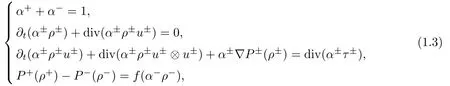
We consider the following compressible nonconservative two- fluid model in R3:

Furthermore,from(1.4)and dP+−dP−=df(α−ρ−),we obtain

Substitute(1.5)into(1.4),we get the following expressions:

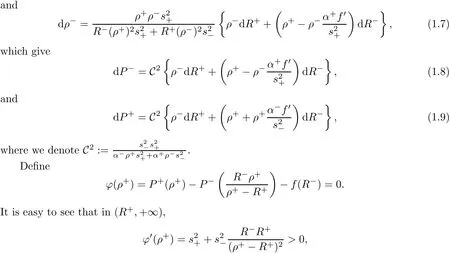
and ϕ:(R+,+∞)7→ (−∞,+∞).

Applying the implicit function theorem to(1.3)4,there exists ρ+= ρ+(R+,R−)such that ϕ(ρ+)=0.Furthermore,we can de fine

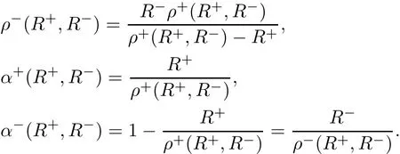
Based on the above,system(1.3)can be rewritten as follows:

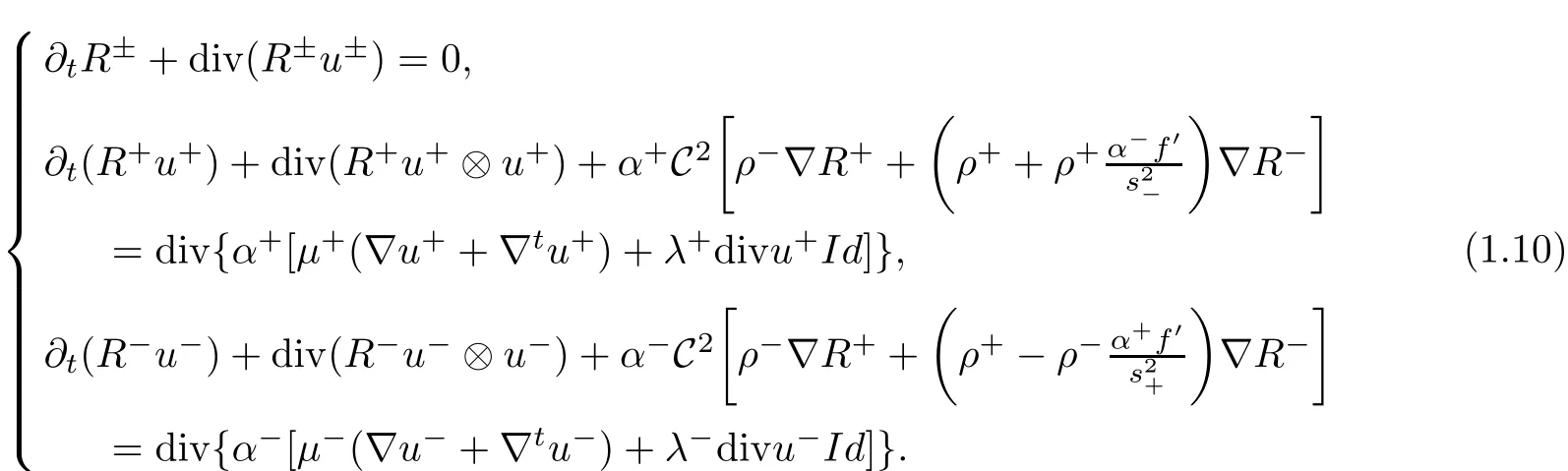
We consider the Cauchy problem of(1.10):

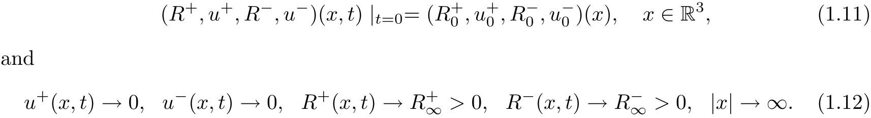
Without loss of generality,we assume.For the above problem(1.10)–(1.11),we obtain the following result.

Theorem 1.1([18],Theorem 1.1)Under the condition

where η is a positive,small fixed constant,there exists a constant ǫ such that if

then the Cauchy problem(1.10)–(1.11)admits a unique solutionglobally in time in the sense that:

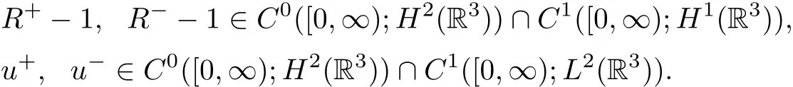
Moreover,if in addition the initial datais bounded in L1(R3),the solution enjoys the following decay-in-time estimates:

Remark 1.2The proof of the theorem involves some new ideas.Usually,the proof consists of spectral analysis of the Green function for the corresponding linearized system and energy estimates of the solutions to the nonlinear system,refer for instance to[7,8].Here,we just need spectral analysis of the low-frequency part of the Green function and the energy estimates.Actually,we employ the energy method in the frequency space to get the decay rates of the low-frequency part so that we succeed to avoid some complicate analysis of the Green function,which is a 8×8 matrix.On the other hand,we notice that the high-frequency part can be handled directly by the energy estimates.Thus,the combination of the decay rates of the low-frequency part and the energy estimates show the decay rates of the solutions directly,even for initial data within the H2-framework.

If the capillary e ff ect is included,we consider the following equations:

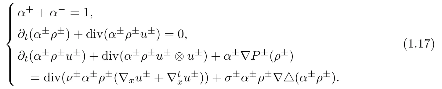
And we consider the two equal pressure functions:.And(1.5)–(1.9)becomes(1.18)–(1.21):

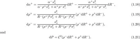
Then the system(1.17)is equivalent to the following form

We consider the problem(1.22)with initial value(1.11)–(1.12).For simplicity,set ν+= ν−= ν,σ+=σ−=σ.Introduce n±=R±−1,then the initial value problem(1.22),(1.11)and(1.12)can be rewritten as

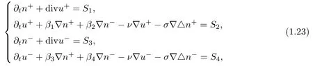
with initial data

and the far- field behavior

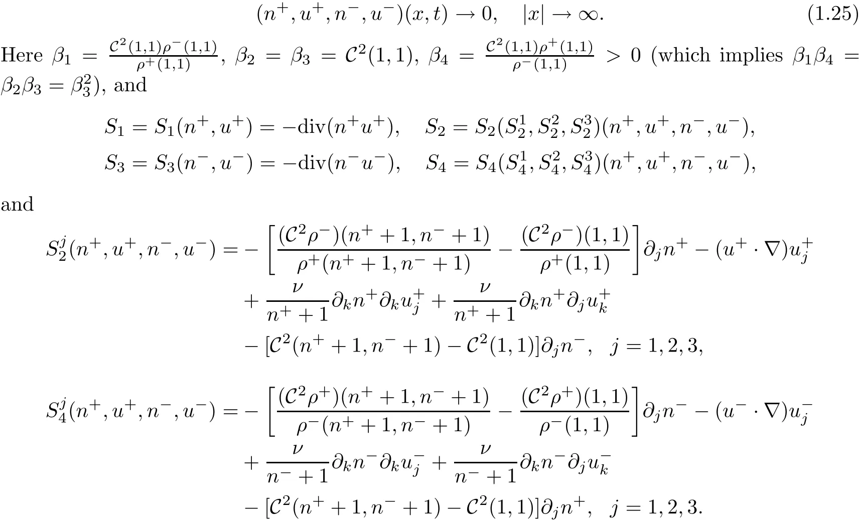
For the above problem(1.23)–(1.25),we obtain the following result.

Theorem 1.3([5],Theorem 1.1) For any integer s ≥ 3,there exists a constant δ>0,such that if

then the initial value problem(1.23)–(1.25)admits a unique solution(n+,u+,n−,u−)globally in time,which satis fies

and for some c,C>0 independent of t such that

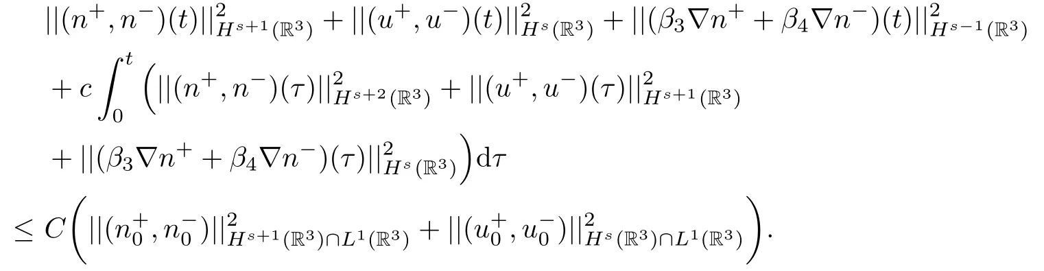
Moreover,the solution satis fies the decay-in-time estimates:

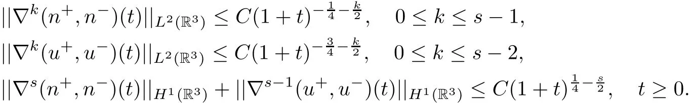
Remark 1.4The fraction densities converge to the equilibrium states at the L2-rate(1+t)−14,and the k(∈ [1,s − 1])order spatial derivatives of the fraction densities converge to zero at the L2-rate,which is slower than theand L2-ratefor the compressible Navier-Stokes system(k=0,1)or Navier-Stokes-Korteweg system(k=0,1,2),see[7,43,49].This is caused by the non-conservation and complexity of the model(1.17).

2 Drift- flux Model

2.1 Research Background-2

The drift- flux model is one of the commonly used models nowadays for the prediction of various two-phase flows.It was first developed by Zuber and Findlay[55].It is used in chemical engineering to predict flow in bubble column reactors,in petroleum applications to model various wellbore operations related to drilling,production of oil and gas,and for the study of geothermal energy related problems and injection of CO2.A one-dimensional transient drift- flux model can be written in the following form:

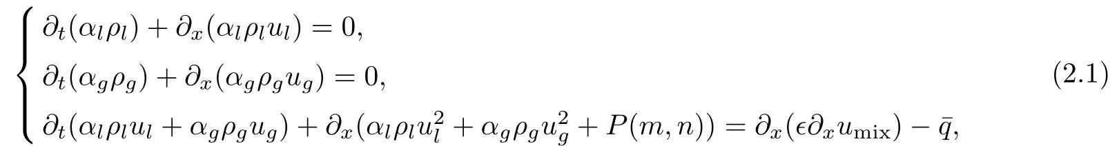
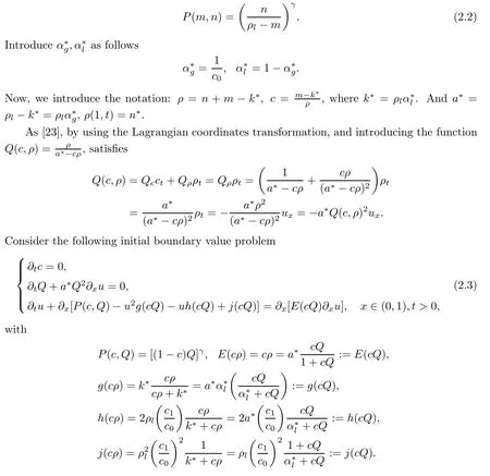
where m= αlρl,n= αgρgdenote the masses of liquid and gas;The unknowns are αl,αg∈ [0,1]volume fractions of liquid and gas,satisfying αl+ αg=1;ρl,ρgthe liquid and gas densities;P=P(m,n)common pressure for liquid and gas;ul,ugvelocities of liquid and gas.In order to get a closed system,an algebraic equation called the slip relation which relates the two fluid velocities is added:ug=c0umix+c1,it implies:

where c0and c1are flow dependent coefficients,c0is referred to as the distribution parameter and c1to as the drift velocity,umix=αgug+αlul;ǫ=ǫ(m,n)(≥0)viscosity coefficient;¯q external force,such as the gravity and frictional force.

For previous studies of the 1D model(2.1)with the slip relationwith c0>1,c1=0,for the free boundary problem,we refer to[10,22].In[10],the local existence of weak solution was obtained whereas[22]gave a local existence of weak solution for a general slip(c0>1 and c1>0)and a global existence result for the special case c0>1,c1=0.The more general case c1>0 is important because it allows the model to describe,e.g.counter-current flow,where uland ugpossibly have di ff erent sign.Recently,Evje and Wen[20]obtained the global existence and unique of strong solution for the 1D initial boundary value problem.This work presents a first global existence result for the drift- flux model with a general slip law.

Next,we give the main well-posedness results about the model(2.1).

2.2 Well-posedness Results

At first,we ignore the external force,i.e.,.Assume that(where b(t)separates the gas-liquid mixture and the gas region,satis fies:b(0)=b0),t>0,and the pressure is given by

Initial conditions are

and boundary conditions are

Assumptions on the parameters α,γ

Assumptions on the initial data

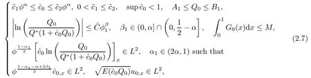
Moreover,the lower bound A of Q and the bound M on the initial energy must satisfy the following relations

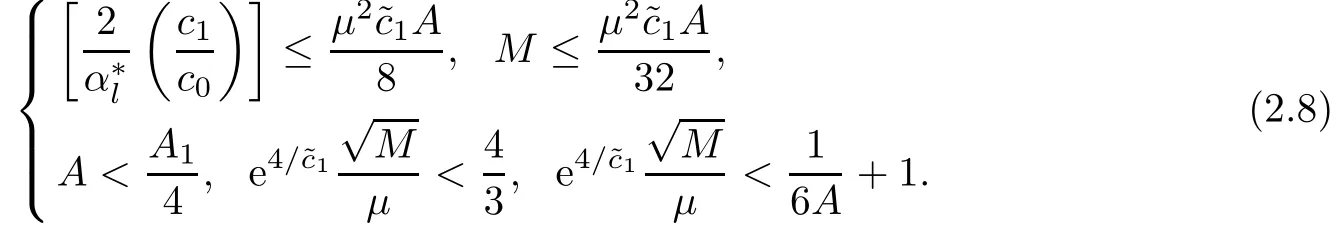
The external pressure p∗must obey

Similarly,the upper bound B of Q and the bound M on the initial energy must satisfy the following relations:

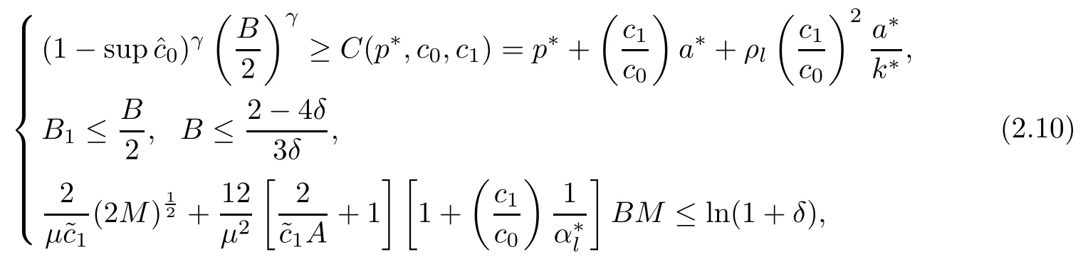
for some δ>0 and subject to the condition sup<1.In addition,A and B are chosen such that:

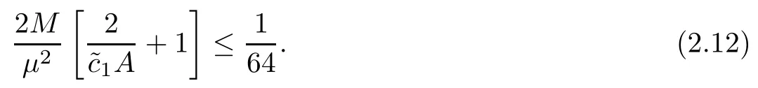
Finally,M must obey the smallness condition as follows:

Theorem 2.1([23],Theorem 2.1(existence)) Under the assumptions of(2.6)–(2.12),there exists a constant M0>0 such that(2.3)–(2.5)admits a global weak solution(c,Q,u)on[0,1]×[0,T]for any time for all M ≤M0in the sense that

(A)The following regularity holhs

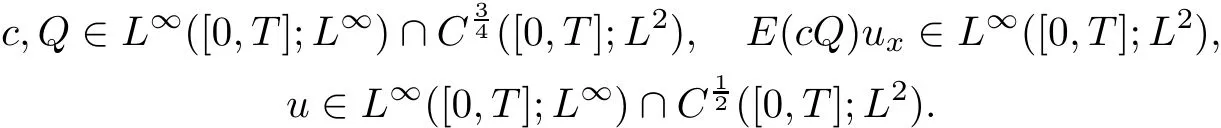
Moreover,the following estimates hold

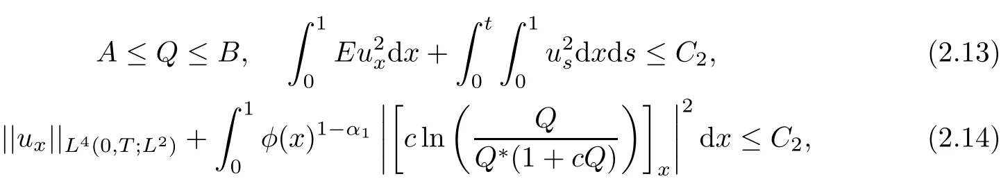
for(x,t)∈[0,1]×[0,T],where C2depends on A,B,M,T and the initial data.

(B)The following equations hold

(C)Interface behavior

for some r∈(1,2)such that r(α+1)<2,and

for β1∈ (0,α]∩(0,−α].Here(x,t)∈ [0,1]×[0,T].

Theorem 2.2([23],Theorem 2.2(uniqueness)) Under the conditions of Theorem 2.1 and by requiring that β1= α,where 0< α ≤,the weak solution is unique.

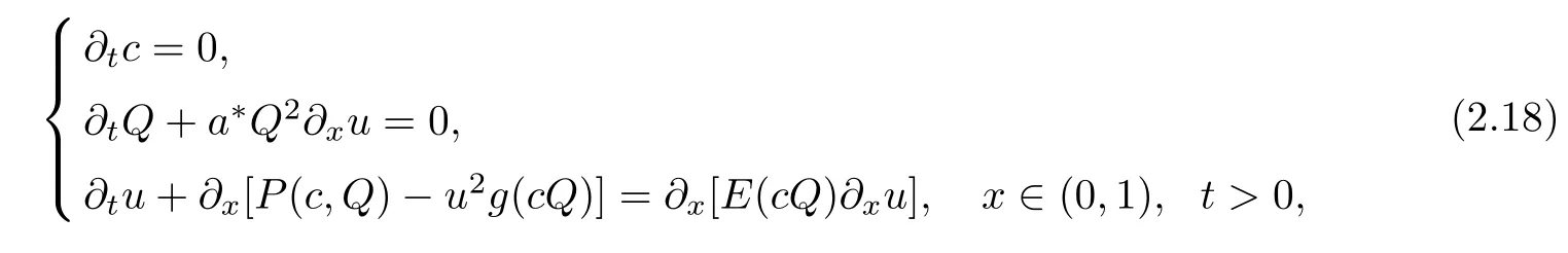
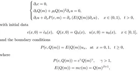
Next,assume that c0≥1,c1=0,x∈(a,b(t)),t>0,i.e.,h(cQ)=j(cQ)=0.Set E(c,cQ)=[cQ]β+1,β >0,and n∗=0(ρ(1,t)=n∗=0).Consider the following initial boundary value problem:

with initial conditions

and with boundary condition

AssumptionsLet A1,B1,and δ be positive constants,whereas α,β>0 and γ>1 such that

where φ(x)=1 − x,and α,β,γ as well as the time decay exponents r1,r2,r3,r4>0,satisfy the following

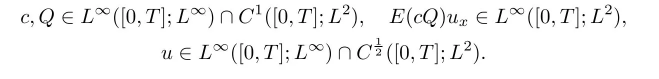
Theorem 2.3([24],Theorem 3.1(global weak solution)) Under the assumptions of(2.21)–(2.22),there exists a positive constant C0such that if δ≤ C0,then(2.18)–(2.20)admits a unique solution(c,Q,u)on[0,1]× [0,∞)in the sense that:

(A)the following regularity holds

(B)the following equations hold

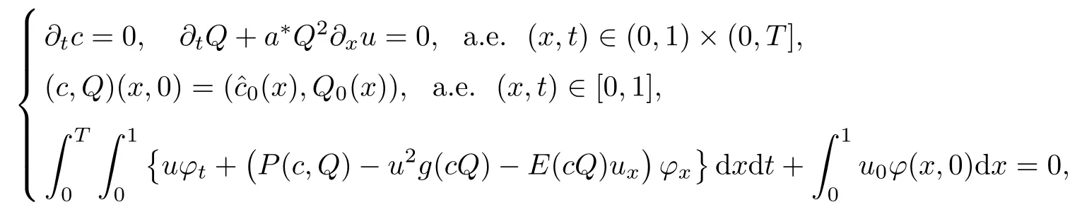
for any T>0 and any test function

In the next section,we will consider the model(2.1)with c0=1 and c1=0,i.e.,ug=ul=u,we call this model as the viscous liquid-gas two-phase flow model.We will use the appropriate variable transformation,to rewrite the model in terms ofwhich is similar to the single-phase compressible Navier-Stokes equations,wheresatis fies a transport equation.

3 Viscous Liquid-gas Two-phase Flow Model

3.1 Research Background-3

Viscous liquid-gas two-phase flow model can be viewed to be simpli fied from the model,which are widely used within the petroleum industry to describe production and transport of oil and gas through long pipelines or well.This model is composed of two separate mass conservation equations corresponding to each of the two phases and one mixture momentum conservation equation in following form

where m= αlρl,n= αgρgdenote liquid mass and gas mass respectively;µ and λ are viscosity coefficients,satisfying:µ >0,λ+≥ 0;The unknown variables αl,αg∈ [0,1]denote liquid and gas volume fractions,satisfying the fundamental relation: αl+ αg=1;Furthermore,ρland ρgdenote liquid and gas densities,respectively;u denotes velocity of liquid and gas;P=P(m,n)is common pressure for both phases,¯q is the external force.

The investigation of model(3.1)has been a topic during the last decade.There are many results about the numerical properties of this model or related model.However,there are few results providing insight into existence,uniqueness,regularity,asymptotic behavior and decay rate estimates concerning the two-phase liquid-gas models of the form(3.1).Let us review some previous works about the viscous liquid-gas two-phase flow model.For the model(3.1)in 1D,when the liquid is incompressible and the gas is polytropic,i.e.,P(m,n)Evje and Karlsen[16]studied the existence and uniqueness of the global weak solution to the free boundary value problem withwhen the fluids connected to vacuum state discontinuously.Evje,Fl˚atten and Friis[13]also studied the model within a free boundary setting when the fluids connected to vacuum state continuously,and obtained the global existence of the weak solution.If the acceleration terms in the mixture momentum equation was neglected,Evje and Karlsen[14]obtained the global existence of weak solution on the half line.If the external force and frictional force were included,see the related results in[27,28].Speci fically,when both of the two fluids are compressible,i.e.,P(m,n)one can consult[15]for the global existence of strong solution to the 1D case;For multidimensional case,Yao,Zhang and Zhu[51]obtained the existence of the global weak solution to the 2D model when the initial energy is small.Furthermore,they proved a blow-up criterion in terms of the upper bound of the liquid mass for the strong solution to the 2D model in a smooth bounded domain,cf.[52].For the Cauchy problem of a multi-dimensional viscous liquid-gas two-phase flow model,Hao and Li[30]obtained the global existence and uniqueness of strong solution for the initial data close to an equilibrium and the local in time existence and uniqueness of the solution with general initial data in the framework of Besov spaces.Concerning the well-posedness and large time behavior of solutions to the model(3.1)and related models,we refer the reader to the[9,11,12,17,29,35,47]and references therein.

Next,we give the main well-posedness results about the model(3.1).

3.2 Well-posedness Results

At first,we consider the model(3.1)in 1D,in order to avoid some unsolved difficulties,we consider a simpli fied model obtained as follows:

(1) Due to the fact that the liquid phase density is much higher than the gas phase density,typically to the order,we can neglect the gas phase e ff ects in the mixture momentum conservation equation.

(2)Neglect the external forces,i.e.,

We assume that further the liquid is incompressible and the gas is polytropic,i.e.,ρl=const,.Then the model(3.1)can be simpli fied into the following model in the form

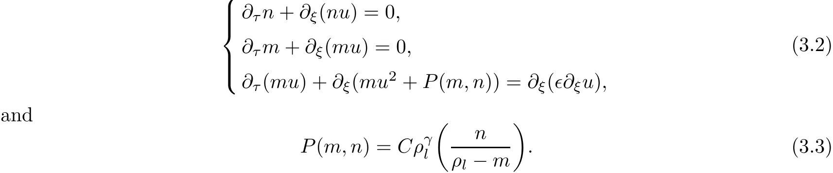
We will consider(3.2)in a free boundary value problem setting where the masses n and m initially occupy only a finite interval[a,b]∈R.That is

and n(ξ,0)=m(ξ,0)=0,ξ∈ R[a,b].The boundary conditions are given as

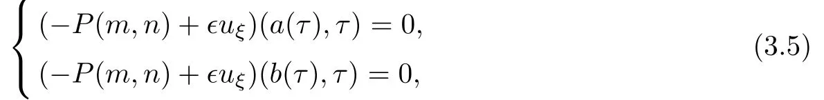
where a(τ)and b(τ)are vacuum boundary,satisfyingu(b(τ),τ),b(0)=b.As in[16],the viscosity coefficient(0,1],k1is a positive constant.In the Lagrangian coordinates,the free boundary value problem(3.2)–(3.5)becomes the following fixed boundary value problem

with initial data

and the boundary conditions

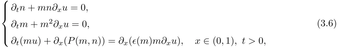
Remark 3.1Introduce the variableswe can rewrite the initial boundary value problem(3.6)–(3.8)in the form

which is similar to the model of single-phase Navier-Stokes equations.Therefore,we can apply technique in studying Navier-Stokes equations to deal with the related problem for the viscous liquid-gas two-phase flow model.

Yao and Zhu[53]improved the previous result of Evje and Karlsen[16]from β∈(0,)to β∈(0,1],and got the global existence of weak solution,regularity of the solutions and the asymptotic behavior result.The result of global existence of weak solution is as follows.

Theorem 3.2([53],Theorem 2.2(Existence and uniqueness)) Under the assumptions of

(A1)

(A2)

(A3) γ>1,0<β≤1,

the initial boundary problem(3.6)–(3.8)possesses a unique global weak solution(n(x,t),m(x,t),u(x,t))satisfying for any T>0

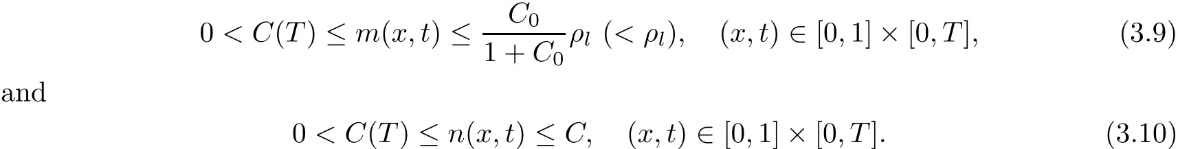
On the other hand,for the viscous liquid-gas model with constant viscosity coefficient when both the initial liquid and gas masses connect to vacuum continuously,Yao and Zhu[54]used a new technique to get the upper and lower bounds of gas and liquid masses n and m,then got the global existence of weak solution by the line method.For this case,the boundary conditions(3.8)is replaced by

Next,we give the de finition of weak solution.

De finition 3.3([54],De finition 1) A pair of functions(n(x,t),m(x,t),u(x,t))is called a global weak solution to the initial boundary value problem(3.6),(3.7)and(3.11),if for any T>0

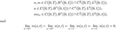
Furthermore,the following equations hold

for any test functions ψ(x,t)∈,with Ω ={(x,t):0 ≤ x ≤ 1,t≥ 0}.

Theorem 3.4([54],Theorem 1) Under the assumptions of

(A1)

(A2)

(A3)is a positive constant and satis fies:

(A4) γ>1,the initial boundary value problem(3.6),(3.7)and(3.11)possesses a unique global weak solution(m(x,t),n(x,t),u(x,t))de fined by De finition 3.3.

Next,we consider(3.1)in 3D.We neglect the gas phase e ff ects in the mixture momentum conservation equation and external force,i.e.,study the following initial boundary value problem

For the problem(3.13)–(3.15),Wen,Yao and Zhu[50]proved the local existence of strong solution and established the blow-up criterion,when there was initial vacuum.If the liquid mass was upper bounded,we could obtain a high integrability of the velocityfor some r∈(3,4].Moreover,in order to overcome the singularity brought by the pressure P(m,n)when there is vacuum,we needed the assumptionwere positive constants.

Theorem 3.5([50],Theorem 1.1(local existence)) Let Ω be a bounded smooth domain in R3and q∈ (3,6].Assume that the initial data m0,n0,u0satisfyare positive constants.The following compatible condition is also valid:

Then,there exist a T0>0 and a unique strong solution(m,n,u)to the problem(3.13)–(3.15),such that

Theorem 3.6([50],Theorem 1.2(blow-up citerion)) Under the assumptions of Theorem 3.5,if T∗<∞is the maximal existence time for the strong solution(m,n,u)(x,t)to the problem problem(3.13)–(3.15)stated in Theorem 3.5,then

Remark 3.7The analysis in Theorem 3.6 can be applied to study a blow-up criterion of the strong solution to compressible Navier-Stokes equations for

which improves the corresponding result about Navier-Stokes equations in[48]where 7µ > λ.

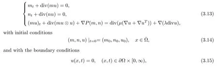
If we don’t neglect the gas phase e ff ects in the mixture momentum conservation equation,and consider the following initial boundary value problem

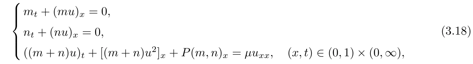
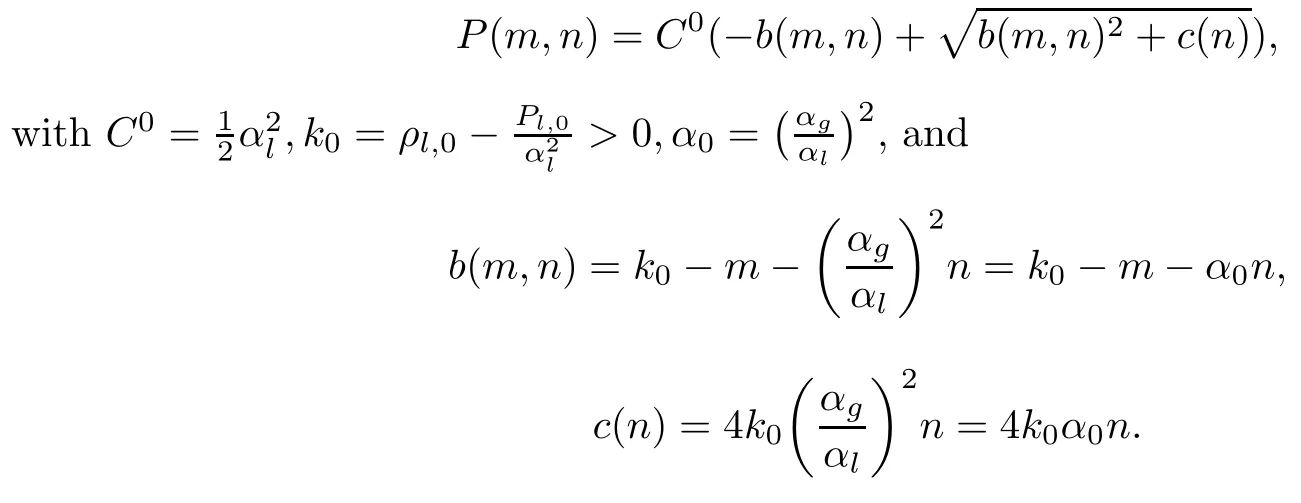
the viscosity coefficientµis constant,the pressure P satis fies

with initial conditions

and with boundary conditions

We give a precise de finition of global weak solutions.

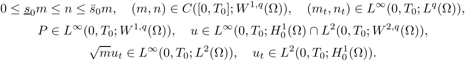
De finition 3.8([26],De finition 1.1) We call(m,n,u):(0,1)×(0,+∞)→R+×R+×R a global weak solution of(3.18)–(3.20)if for any 0

(1)m,n∈L∞((0,1)×(0,T)),(m+n)u2∈L∞(0,T;L1(0,1)),m,n≥0 a.e.,in(0,1)×(0,T),u∈L2(0,T;

(2)(m,n,u)satisfy the system(3.18)in the sense of distribution;

(3)(m,n,(m+n)u)(x,0)=(m0(x),n0(x),M0(x)),a.e.x∈(0,1).

Theorem 3.9([26],Theorem 1.1(global existence))then there exists a global weak solution(m,n,u):

Remark 3.10Note that we do not need the conditionsfor sometypically made use of in previous literature[15,50–52].This implies that transition to single phase is allowed,i.e.,one of the two phases can completely occupy some regions.

4 Open Problems

•Compressible nonconservative two- fluid model

Compared with the single-phase flow(i.e.,compressible Navier-Stokes equations),the twofluid model has its own challenges by means of the nonconservative structure in the pressure terms.More speci fically,when one looks for the global solutions with large initial data in the sense of distribution,the spatial derivatives in the pressure terms can not all be shifted to the test functions.In view of the fact,one has to obtain some estimates of the spatial derivatives of density or the related.This makes that two viscosity coefficients have to be equivalent to the corresponding density,i.e.,,see[3]for 1D case.To our best knowledge,it is still open for the case of multi-dimensions and for thatwith more general α,β ∈ [0,∞).

•Drift- flux model

The main di ff erence between two- fluid model and drift- flux model is that two fluids are considered as a whole in the momentum equations for the latter case.However,in this case,some other equations have to be added to the system for completeness.The so called“slip law”is commonly used.The main challenge is that the global entropy estimate is difficult to find though the momentum equation is of the conservative form.This leads to an open problem whether the global weak solutions with large initial data exist or not for more general slip law.In fact,when c0=1 and c1=0 for large initial data,and c0≥1,c1≥0 for small initial data,it is known that the global weak solutions exist,see[26],and Theorems 2.1 and 3.2 respectively.Here c0and c1are constants.

•Viscous liquid-gas two-phase flow model

The viscous liquid-gas two-phase flow model can be considered as a simpli fied case from the two- fluid model when two velocity fields and two pressure functions are equal respectively.Although there are some results achieved for the simpli fied case particularly,there are still some open problems.For example,whether the global smooth solution with large initial data in high dimensions exists or not,or equivalently whether the smooth solution blows up in finite time.