Xiang-rui Dong (董祥瑞), Yi-qian Wang(王义乾), Xiao-ping Chen(陈小平), Yinlin Dong,Yu-ning Zhang (张宇宁), Chaoqun Liu

1. National Key Laboratory of Transient Physics, Nanjing University of Science and Technology, Nanjing 210094,China

2. Department of Mathematics, University of Texas at Arlington, Arlington, Texas, USA

3. School of Aerospace Engineering, Tsinghua University, Beijing 100084, China

4. School of Mechanical Engineering, Zhejiang Sci-Tech University, Zhejiang 310018, China

5. Department of Mathematics, University of Central Arkansas, Conway, Arkansas, USA

6. Key Laboratory of Condition Monitoring and Control for Power Plant Equipment (Ministry of Education),School of Energy, Power and Mechanical Engineering, North China Electric Power University, Beijing 102206,China

7. Beijing Key Laboratory of Emission Surveillance and Control for Thermal Power Generation, North China Electric Power University, Beijing 102206, China

Abstract: In the present paper, epsilon ()ε in the Omega vortex identification criterion (Ω method) is defined as an explicit function in order to apply the Ω method to different cases and even different time steps for the unsteady cases. In our method, ε is defined as a function relating with the flow without any subjective adjustment on its coefficient. The newly proposed criteria for the determination of ε is tested in several typical flow cases and is proved to be effective in the current work. The test cases given in the present paper include boundary layer transition, shock wave and boundary layer interaction, and channel flow with different Reynolds numbers.

Key words: Vortex identification, vorticity, deformation, turbulence

The definition or identification of vortex is a longstanding issue in fluid dynamics. Several vortex identification methods, such as Δ~-method[1], Q[2]and2λ[3]criteria have been widely used to capture vortex structures in turbulent boundary layers of DNS data[4]. However, in order to capture the vortex, a threshold is generally required in the aforementioned methods. However, a proper choice of the threshold is still quite illusive, leading to many limitations.Recently, Zhang et al.[5]reviewed various kinds of existing vortex identification methods in the literature,and classified the methods into several different groups. In many existing methods, a selection of the threshold for the vortex identification is necessary.Hence, an improper threshold could lead to incorrect results. A new Omega method （Ω）, firstly proposed by Liu et al.[6], appears to overcome those weaknesses.Recently, Zhang et al.[5]applied this new Ω method into the analysis of the reversible pump turbine and indicated that this new omega method is quite suitable for the analysis of the inner flow of hydro-turbines,especially the complex flow cases. Tao et al.[7]also utilized this Ω method to investigate the wake flow of the moving bodies in their study, and they pointed out that comparing to other vortex identification methods, the new Ω method has a clear physical meaning. The Ω method has also been used by other researchers[8-9]to compare with the existing vortex identification methods. Different with most of the existing vortex identification methods with an absolute threshold, the new Ω method employs a determinative value to capture the vortex with a normalized value ranging from 0 to 1. Meanwhile, Ω has a clear physical meaning through defining the vortices with the vorticity overtaking the deformation.Vorticity can directly represent the rotation of a solid body, but not that of fluid. In other words, vorticity not only represents the fluid rotation, but also the fluid deformation. Therefore, the basic idea of the Ω method is that a ratio of vorticity and deformation is employed to measure the rotation level. The pure deformation can be defined as flows with Ω=0 while the rigidly rotational flow is defined as flows with Ω=1. However, no previous literature gives a detailed study on an involved significant parameter in the new Ω method, named as Epsilon ()ε. In this study, the determination of ε in the new Ω method is discussed and compared with different values of ε and also the widely employed Q criterion. Several examples are presented to demonstrate the validities of the present work.

1. ε determination

In order to study the significance of the parameter ε and also determine its value, the Ω method is reviewed in this section. Although rigid body rotation must possess vorticity, vorticity cannot directly represent the fluid rotation. Therefore, in fluid flow, the vorticity could be small in a strong rotation and could be large in a weak or zero rotation. The laminar boundary layer flow by Blasius solution is a typical example. For the vortex flow, deformation is also an important factor in a rotational flow. Therefore,for a physical definition of the vortex, it is reasonable to consider the ratio of the vorticity and the deformation. As given in our previous papers[6,10-12]and also shown in Eq. (1), Ω is defined as a ratio of vorticity squared over the sum of vorticity squared and deformation squared

where A is the symmetric part of the velocity gradient tensor ∇V, B is the anti-symmetric part,is the Frobenius norm.

In the practical application, we pick

where

It should be noted that the ε in Eq. (4) is a small positive number used to avoid division by zero[6].However, in the previous Ω method[6], the non-dimensional typical length scales and velocity must be employed in order to calculate Ω with a proper choice of ε. This could be an obstacle to many users of the Ω method.

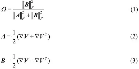
Fig. 1 Boundary layer transition iso-surfaces of Ω=0.52 with different ε levels

Although Ω is non-dimensional and satisfies Ω∈[0,1], some serious noises (clouds) may appear inside the flow domain if both term a and b in this ratio (Eq. (1)) are in close proximity to zero due to the systematic computational errors. These noises can be reduced or even removed by introducing a proper positive number of ε in the denominator of Ω as shown in Eq. (4). Therefore, in the present method,the new method for the determination of ε is introduced to remove the noises caused by the consequence of division by zero. Apparently, as a small number, ε is dependent upon the dimension of the physical variables and needs to be adjusted to be a proper number case by case and time by time. Based on the description of the above issues, the determination of ε is a critical issue for the application of Ω method. In our current study, a linear correlation is found between ε and the maximum of b-a. The ε is defined as a function of (b-a)max, which is a fixed parameter at each time step in each case. In this study, ε is proposed as follows

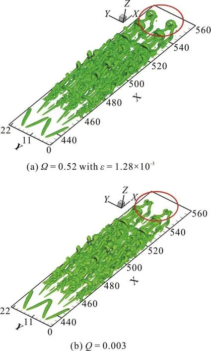
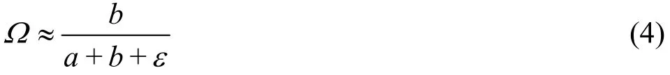
Fig. 2 Boundary layer transition iso-surfaces at t=8.2T

It should be noted that Eq. (5) is an empirical formula based on a large number of test results from different cases. The term (b-a)maxrepresents the maximum of the difference of vorticity squared and deformation squared, and could be easily obtained as a fixed number at each time step in a certain case.

2. Comparisons with Q criterion

In this section, the Omega method is compared with the Q criterion. Actually, as stated below, Ω has many essential differences with the Q criterion or other similar methods (e.g. the kinematic vorticity number[13]).

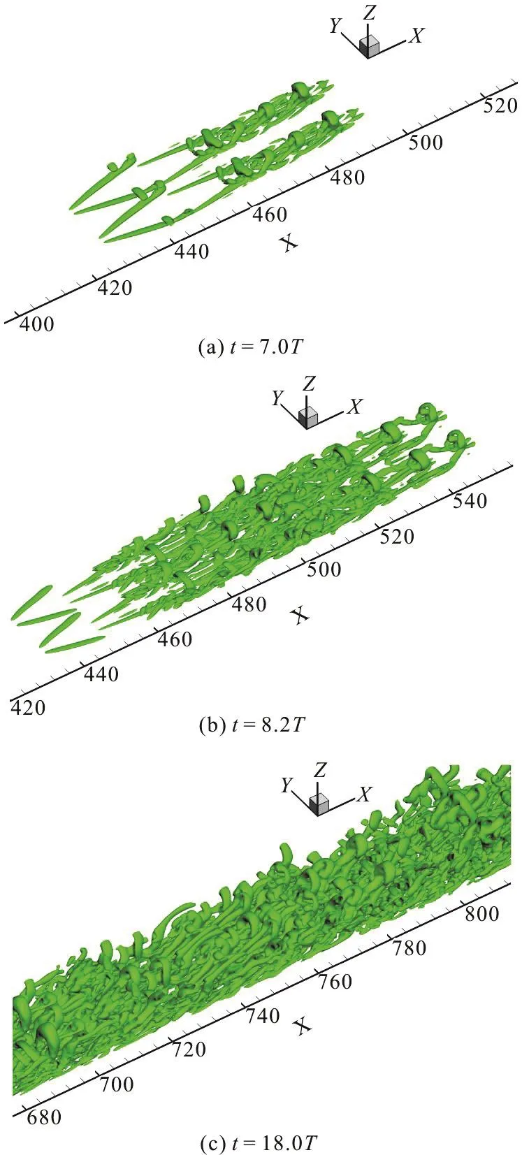
Fig. 3 Boundary layer transition iso-surfaces of Ω=0.52 at different time steps

On the one hand, Q is a special situation of Ω when Ω=0.5 and ε=Qth, where Qthis a certain number picked from a series of varying thresholds by experience. For instance, if we pick Ω=b/( a+b+Qth)=0.5, b-a=Qth. Hence, both Ω=0.5 and Q=Qthwill give exactly the same results. However,for most general cases, the new Ω method is essentially different with the Q criterion.

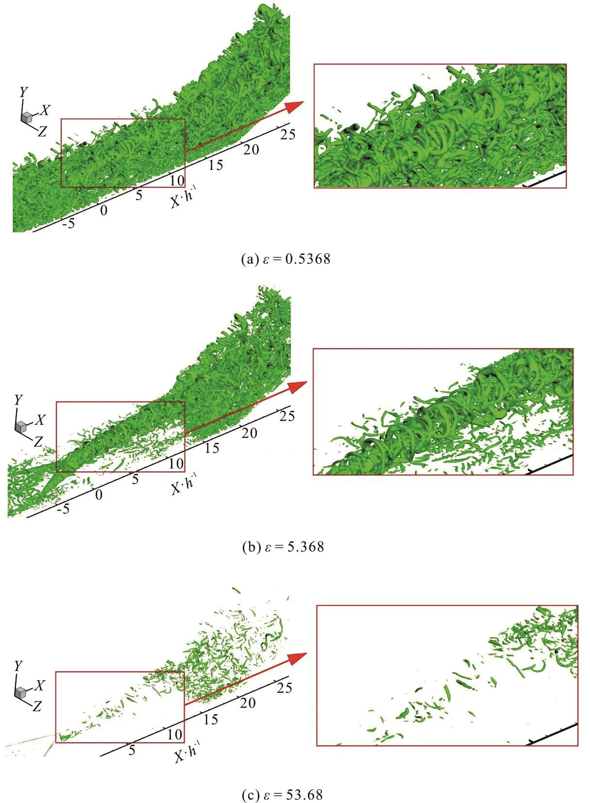
Fig. 4 Iso-surfaces of Ω=0.52 with different ε levels in case 2

On the other hand, Ω method can capture both strong and weak vortex structures simultaneously by setting Ω=0.52 but Q criterion may not[10]. Ω denotes a ratio ranging from 0 to 1, which represents the rotational quality of the vorticity. For instance, for weak vortices, the value of Q or 0.5(b-a) may be very small. When choosing a large value of Q, the weak vortices will be lost with only strong vortices left. However, no matter how weak these vortices are,they are always well shown in the region where the vorticity overtakes the deformation. Alternatively, if we reduce Q to show the weak vortices, the strong vortices may be smeared and cannot be visualized clearly.

3. Application examples of a newly determined ε method

To verify the above ε determination method, a number of several typical computational examples are presented and analyzed in this section. Different ε levels are tested for case 1 and case 2 at different time steps. Meanwhile, the Ω method with the new ε determination is also utilized in case 3 and case 4 for the comparison with the Q criterion.

3.1 Case 1: Boundary layer transition

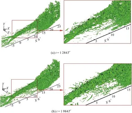
Fig. 5 Iso-surfaces of Ω=0.52 at different times in case 2

A Mach 0.5 boundary layer transition on a flat plate based on high order direct numerical simulation(DNS) is chosen as Case 1 to test the new ε determination method. The grid system is nstreamwise×nspanwise×nnormal=1920× 128× 241. Firstly we give a comparison of different ε levels at t=8.2T, where T is the period of T-S wave. ε is chosen as 1.28×10-3based on the new ε determination in Eq.(5). Figure 1 shows the iso-surfaces of Ω=0.52. As clearly shown in Fig. 1, with smaller ε, there are too many clouds (noises) in Figure 1(a) which is marked in a red square. However, some significant vortex structures cannot be shown with a larger ε (Fig.1(c)). For instance, in the downstream region marked in a red square in Figure 1(c), the vortex rings disappear compared with the one in Figure 1(b).Therefore, for this case, the ε based on the new ε function is proper to be used in vortex identification given by Ω=0.52.

Furthermore, Ω has been reported to have a capability of well capturing both strong and weak vortex structures simultaneously in our previous work[6]. In current work, =0.52 Ω with newly determined ε still inherits its advantage. The isosurfaces of Ω=0.52 with ε=1.28× 10-3and Q=0.003 at t=8.2T are compared in Fig. 2.Q=0.003 is chosen for comparison with Ω=0.52 since it shows the same strong vortex surfaces in the upstream of the transition flow. However, as can be seen in the red circle of Fig. 2, the vortex rings in the downstream of the flow especially their heads cannot be captured by Q=0.003. That means a larger Q may le ad to we ak vort ices disa ppear altho ugh the m ain strongvorticescouldbestillcaptured.However,if Alternatively, if one adjust Q to be a smaller value,the weak vortices are captured but strong vortices are smeared.

On the other hand, the new determination of the ε is also tested in different time steps of case 1.Figure 3 shows the iso-surfaces of Ω=0.52 at different time steps. The newly determined ε in each time step is listed in Table 1 accordingly. As shown in Table 1, a typical vortex structures are well captured in different time steps without noises appearing in the space. Note that one do not need to adjust the ε to be a proper value for different time steps. During the vortex identification in different time steps, one could calculate the ε using the values ofmax(b-a)obtained in each time step as shown in Eq. (5).

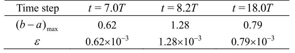
Table 1 New ε determination at different time steps in case 1

3.2 Case 2: SWBLI controlled by MVG

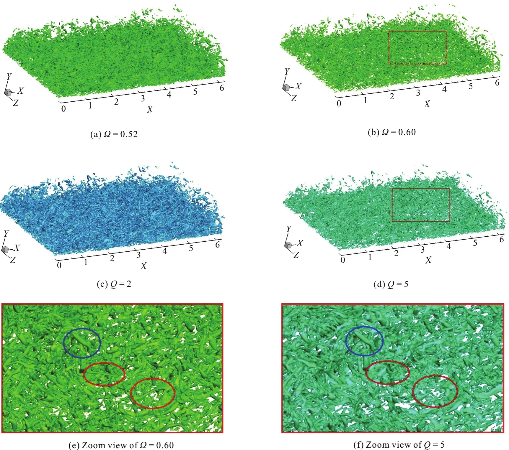
Fig. 6 Different iso-surfaces in case 3 with different values of Ω and Q

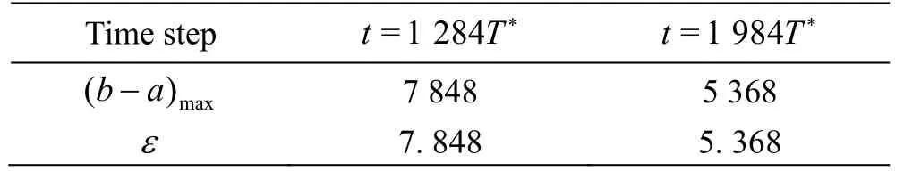
Table 2 New ε determination at different time steps in case 2

The shock wave and boundary layer interaction(SWBLI) in a supersonic ramp flow with MVG control at Mach number 2.5 is selected as case 2. In this case, the simulation was accomplished by the implicitly implemented LES (ILES) method. The body-fitted grid system of the computational domain is nstreamwise×nspanwise×nnormal=1600× 192× 137. Similarly, the iso-surfaces of Ω=0.52 with different ε levels for the case 2 at t=1 984T*are compared in Figure 4, where T*is the characteristic time in case 2. The newly determined ε is 5.368 since (b-a)maxis 5,368 at t=1 984T*and the corresponding iso-surface is shown in Fig. 4(b). As shown in Fig.4(b), the vortex rings behind MVG are visualized and even the number of the rings can be clearly counted.However, the vortex rings may not be clearly captured in Fig. 4(a) with ε=0.5368, due to too many small-scale structures around them. In Fig. 4(c)with ε=53.68, the large vortex structures like vortex rings a re absent fr om the domain, and only small-scale vortexstructuresaredemonstrated,whichmakesit meaningless for the analysis of the MVG control.

Figure 5 shows the iso-surfaces of Ω=0.52 with the newly determined ε at different times. The term(b-a)maxand the newly determined ε in each time step are listed in Table 2, respectively. At different time steps, it can be observed that the strong vortex structures like vortex rings are well captured without any clouds in the upper space of the vortex rings.

3.3 Case 3: Channel flow with Reτ=950

The new ε determination of the Ω method is tested in a turbulent channel flow with Reτ=950(case 3), and the comparison with Q criteria is also shown here. The computational domain is 2π×π×2 with 768×768×385 grid points in the streamwise,spanwise and normal directions, respec- tively. Half domain in the normal direction is employed due to the symmetry condition given in the simulation. For the computational details, readers are referred to Lozano-Duran and Jimenez[14].

The compari sons between Ωme thod with new ε determinationand Q criteriononcapturing the vortex structures in this channel flow are given in Fig.6. Figures 6(a) and 6(b) show the iso-surface of Ω=0.52 and Ω=0.60, where the newly determined ε is 2.9698. Figures 6(c) and 6(d) show the iso-surface of Q=2 and Q=5. As shown in the figure, similar vortex structures can be captured by the iso-surfaces of Ω=0.52 and Q=2, as well as the iso-surfaces of Ω=0.60 and Q=5. However, it is convenient to obtain both strong and weak vortex structures by Ω=0.52 with ε=0.001(b-a)max,while the adjustment of Q is needed due to its uncertainty of the threshold. In addition, although a similar vortex structures can be captured by Q=2 after its adjustment, we still do not know the clear physical meaning of Q=2. However, Ω ranges from 0 to 1, and represents the dominance of the fluid rotation and Ω is set as 0.52 for capturing both strong and weak vortices.

In addition, Figs. 6(e) and 6(f) give a zoom view of Figs. 6(b) and 6(d). In Figs. 6(e) and 6(f), the same strong vortex structures could be both captured by Ω and Q referring to the blue circle. However, it is found that some weak vortices (with the red circle) are lost by using Q.

3.4 Case 4: Channel flow with Reτ=451

Another compressible turbulent channel flow[15-16]with Reτ=451 is tested as case 4 for the validation.The computational domain is 4π×4π/3×2 with the grid system of nstreamwise×nspanwise×nnormal=571× 251×261. Figures 7(a) and 7(b) show the 3-D view and the top view of a half normal channel flow by the iso-surfaces of Ω=0.52 and Q=0.2. In Fig. 7(a),the term (b-a)maxis 161.98, thus, the newly determined ε is around 0.162. From the Fig. 7,similar vortex structures can be recognized by Ω=0.52 and Q=0.2. However, the iso-surface with Q=0.2 is selected through adjusting the Q values many times in order to fit the results with Ω=0.52. Whereas, with the present method for the ε determination, Ω can always be set as 0.52 for capturing both strong and weak vortices without any subjective adjustment of both itself and ε.

4. Conclusions

In this study, the new definition and determination of ε are proposed in order to improve the Ω vortex identification method as follows.

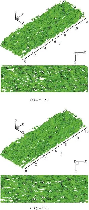
Fig. 7 Iso-surfaces for a channel flow (the upper plot for the 3-D view and the downward plot for the top view).

(1) The new method for the determination of ε in the denominator of Ω is easy to perform, since ε does not need to be adjusted from an arbitrary threshold but can be calculated as a proper and a fixed number depending on the term (b-a)max.

(2) Ω indicates a region where vorticity overtakes deformation in a flow field and could capturing both strong and weak vortices simultaneously. It is difficult to obtain the accurate surface of vortex structures by Q, λ2or other criteria since their thresholds vary in different cases.

(3) Ω method is quite robust with no obvious change in the vortex visualization when Ω varies from 0.52 to 0.60.

Presently, the new omega method has been widely employed for the vortex identification in various kinds of industrial-level flows (e.g., reversible pump turbine[17]). In the future, the new Ω method will be further applied to a more broad range of complex flows for the purpose of vortex identification e.g. wind turbine[18], hydroturbines[19-20], cavitating flow[21-23], silt-laden flow[24], pumps[25-27], acoustic bubbly flow[28-29], and pressure wave induced flow[30].

Acknowledgements

This work was supported by the Department of Mathematics at University of Texas at Arlington. The authors are grateful to Texas Advanced Computing Center (TACC) for the computation hours provided.This work is accomplished by using Code DNSUTA released by Prof. Chaoqun Liu at University of Texas at Arlington in 2009.