Bin-Quan Li(李斌全)and Sheng-Jun Wang(王圣军)

School of Physics and Information Technology,Shaanxi Normal University,Xi’an 710119,China

1 Introduction

Self-organized criticality(SOC)is a key concept as a possible explanation for the widespread occurrence in many nature systems that long range correlations in space and time.[1−5]Earthquakes are probably the most relevant paradigm of SOC that can be observed by humans on earth.The relevance of SOC to earthquakes was first pointed out by Bak,Tang,and Wiesenfeld,[1]Sornette and Sornette.[6]According to this theory,plate tectonics provides energy input at a slow time scale into a spatially extended,dissipative system that can exhibit breakdown events via a chain reaction process of propagating instabilities in space and time.The empirical Gutenberg-Richter(GR)law[7]arises from the system of driven plates building up to a critical state with avalanches of all sizes.According to the GR law the distribution of earthquake events is scale free over many orders of magnitude in energy.

Then Olami,Feder and Christensen(OFC)introduced a nonconservative model on a lattice that displayed SOC.[8]The OFC model of earthquakes has played an important role in the context of SOC since 1992.However,the presence of criticality in the nonconservative version of the OFC model has been controversial since its introduction and it is still debated.[9−13]

OFC models on different topologies have been investigated in the papers,such as,the annealed random neighbor(ARN)graph model,[14−17]the OFC model on a quenched random(QR)graph[18]and the effects of smallworld and scale-free topologies on the criticality of the non-conservative OFC model.[19−24]

Most work in this area is usually focused on their topological properties[25−29]and homogeneous lattices with or without periodic boundary conditions.But the real systems modeled by these objects are not homogeneous.In a geological fault,for example,the local friction between the moving plates,which in fl uences both the rate of motion and the redistribution on the neighbors in the OFC model,cannot be expected to be a constant value but should fl uctuate according to local variations.Similarly,the local elasticity of the sheets,which determines how the energy is transferred from one point to another,is also expected to be variable.Therefore,a first step is to simply see how the introduction of quenched disorder in the simple coupled-map representation for these systems will affect their dynamical behavior.Some work has already been done along these lines.

A new earthquake model based on a random network was studied,on which the toppling mechanism of the system is that the force of the unstable site is redistributed to their nearest neighbors randomly.[30−32]It is shown that when the system is conservative,the probability distribution displays power-law behavior.However,it displays no scaling behavior when the system is nonconservative.It is like the results in the ARN OFC model.But it is quite different to the model on quenched random graph[18]and the model on square lattice,both of which display criticality even the system is dissipated.It seems that the toppling mechanism of the system has affected the critical behavior of the system.They also compare the critical behavior of the model with different number of nearest neighbors.It is shown that different spatial topology does not alter the critical behavior of the system.

Mousseau studied the in fl uence of quenched disorder on a coupled map model of earthquakes.[33]In his work,disorder is introduced in the redistribution fractionαiwhich now varies from site to site asαi=α+δi,whereδiis a random number taken from a linear distribution[−δ,δ].He said that the question of the role of disorder in dynamical systems is fundamental because most biological,neurological,or geological dynamical systems evolve in the presence of one or another type of disorder.

Janosi and Kertesz studied the effect of randomness in the threshold for the OFC rule.[34]They found that this type of disorder destroys criticality and changes the distribution of avalanche size from power law to exponential.

Ceva looked at uncorrelated and correlated disorder in the redistribution parameterα.[35]He was interested,however,in the effects of concentration of defects and not their amplitude.He found that SOC is stable under small concentration of defects.

In this work,we investigate the critical behavior on a modi fied anisotropic OFC model.Two situations are considered in this paper.One situation is that the energy of the unstable site is redistributed to its nearest neighbors randomly not averagely and keeps itself to zero.The other situation is that the energy of the unstable site is redistributed to its nearest neighbors randomly and keeps some energy for itself instead of reset to zero.Different boundary conditions are considered as well.The rest of the paper is organized as follows.In Sec.2,we review the original OFC model and we point out the main reasons that have induced us to study the modify OFC model.In Sec.3,we investigate the modi fied model and make comparison with other models by analyzing the distribution of earthquake sizes.Finally,in Sec.4 we provide brief discussion and conclusion.

2 Model

The OFC model is de fined on a two-dimensional square lattice ofL×Lsites.Each site is associated a real continuous energyEi.To mimic that the system is driven continuously and uniformly,the value ofEiincreases at the same rate.In simulations, find the largest value of energyEmaxin the system and increase the energy of all sites by the same amountEth−Emax.Therefore,the sites with the largest energy reaches the threshold value(Ei≥Eth)and becomes unstable.As soon as a site becomes unstable,i.e.,Ei≥Eth,the global driving is stopped and the system evolves according to the following local relaxation rule

where“nn” stands for the collection of nearest neighbors to nodei.In general,there are 4 of nearest neighbors,and only the isotropic situation is considered.The parameterα∈[0,1/4]controls the level of conservation of the dynamics,whereα=1/4 corresponds to the conservative case,whileα<1/4 implies the model is nonconservative.

The toppling of one site triggers an avalanche,that is,neighbors of this site may become unstable and toppling propagates in the network.The avalanche is over until all the sites are belowEth.Then the driving to all sites recovers.The number of toppling sites during an earthquake is de fined as the earthquake sizeS.Open boundary condition is used in OFC model.[36]

Here we modify the OFC model only in the toppling rule:when there is an unstable site toppling,the energy of the site is redistributed to its nearest neighbors randomly not averagely as follows.

If anyEi≥Eththen redistribute the energy onEito its neighbors randomly according to the following rule

where“nn” stands for the collection of nearest neighbors to nodei,qis the number of nearest neighbors of every site.The anisotropic situation is considered in this modi fied OFC model.The size of parameterβnnis different for nearest neighbors.The parameterβ∈[0,1]controls the level of conservation of the dynamics that is equivalent to 4αin the OFC model,whereβ=1 corresponds to the conservative case,whileβ<1 implies the model is nonconservative.The parameterβnnat each site is chosen randomly from a uniform distribution between 0 andβ,and the sum is equal toβ.Details as follow,

The other model that differs from above model only in the toppling rule:when there is an unstable site,the energy of the site is redistributed to its nearest neighbors randomly and keeps some energy for itself instead of reset to zero,that is not Eqs.(2),(3)but Eqs.(4),(5),as follow

where“nn” stands for the collection of nearest neighbors to nodei,qis the number of nearest neighbors of every site.β00is de fined as follow

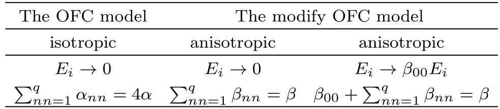
Table 1 The different of the two models.

To completely de fine the model,we need to consider the boundary conditions.We care about the open and periodic boundary conditions in our models.[36−39]The energyαEof an unstable site at boundary is lost in the case of open boundary conditions.Periodic boundary conditions mean the energy is not lost,it is transferred to the other side,like a ring.In Table 1,we list the different of those models to be clearly understood.

In a system of SOC,the distribution of earthquake sizes is a power law function.The power-law exponentτis de fined as

In simulation,we will be interested in the distribution of avalanche sizesP(S).

3 Simulations and Results

3.1 The One Case of the Modi fied OFC Model

Now we study the one case of the modi fied OFC model(Case 1).The energy of the unstable site is redistributed to its nearest neighbors randomly not averagely and keeps itself to zero.In comparison to the original OFC model we plot the distribution of avalanche sizes in Fig.1.The statistics are collected in the critical state for 109non-zero avalanches for each system size.

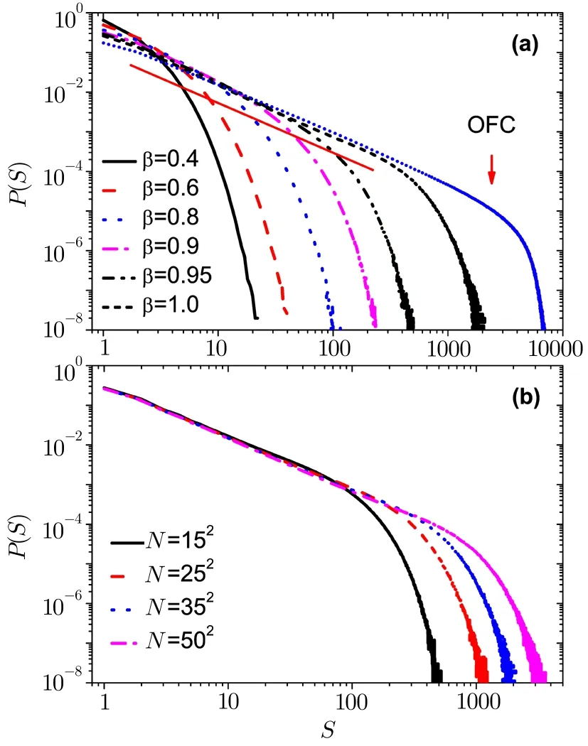
Fig.1 (Color online)Avalanche size distribution with open boundary conditions for(a)different the value of the parameter β with the system size N=352.Different curves correspond to β=0.40,0.60,0.80,0.90,0.95,and 1.0,from left to right.For comparison purposes,the original OFC model of α=0.25 is shown in the direction of the arrow.(b)Distribution of earthquake size for the different system size with β=1.0.

In Fig.1(a),we show that the earthquakes size distributionP(S)for different values of the dissipation parameterβ,in the network withN= 352and with open boundary conditions.Different curves correspond toβ=0.40,0.60,0.80,0.90,0.95,and 1.0,from left to right.We can see that the model transits from non-SOC to SOC behavior with the increase of the parameterβ.Power-law fit is shown as red solid line,the slope of the straight line isτ=1.286 58 forβ=1.0.It is like the critical exponent of the original OFC model.For comparison purposes,the original OFC model ofα=0.25 is shown in the direction of the arrow.

In OFC model,the SOC states exhibit that the distribution is a power law function with an exponential cuto ff.The largest avalanche size in OFC model is about 7000.In the modi fied OFC model,the distribution of avalanche size depends on the dissipation parameterβ.The largest avalanche size in modi fied OFC model is about 1000,which is close to the system sizeN.

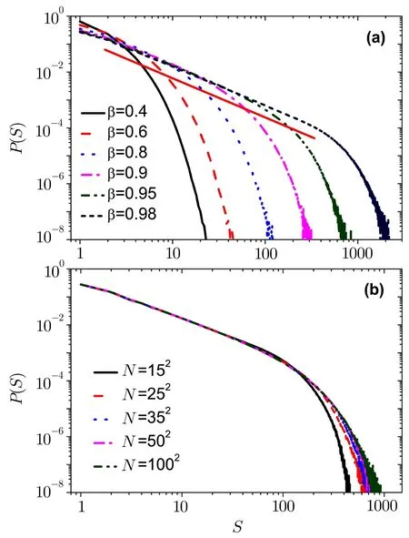
Fig.2 (Color online)(a)Simulation result for the probability density of having an earthquake of energy E as a function of E for a dissipation parameter β with N=352 and with periodic boundary conditions.Different curves correspond to β=0.40,0.60,0.80,0.90,0.95,and 0.98,from left to right.The fitted curve is shown as red solid line.(b)Distribution of earthquake size for the different system size with β=0.95.Different curves correspond to N=152,252,352,502,and 1002.

It is not like the result of the original OFC model.The original OFC model exhibits SOC behavior for a wide range ofαvalues and the exponentτdepends onα.However,we find that this modi fied OFC model exhibits power law distribution when the value ofβtends to 1.It is similar with the model on RN[14,16]and small-world networks.[19,23−24]

In Fig.1(b),we show that the earthquakes size distributionP(S)for different size of the systemN,different curves correspond toN=152,252,352,and 502,from left to right.Size effect is present in Fig.1(b).It is like the result of the original OFC model.The scaling of the cutoffin the energy distribution as a function of the system size forβ=1.0.

Now we plot the distribution of earthquake size for different values ofβwith periodic boundary conditions.As shown in Fig.2(a),we noticed that the model transits from non-SOC to SOC behavior with the increase of the dissipation parameterβ.Power-law fit is shown as red solid line,the slope of the straight line isτ=1.397 15 forN=352andβ=0.98.The largest avalanche size is about 103in the modi fied OFC model withβ<1.0.Although the system size isN=352,the largest size of avalanche is very large with periodic boundary conditions andβ=1.0.The largest size of avalanche is 108much larger than 103.There is not much difference in the results under different boundary conditions,except inβ=1.0.The result is only a slight difference in the critical exponent.As shown in Fig.2(b),the simulation results of avalanche size distribution in systems with dissipation parameterβ=0.95 and network sizeN=152,252,352,502,and 1002,respectively.Although system sizes range from 152to 1002,the change of the largest size of avalanche is very small.

3.2 The Other Case of the Modi fied OFC Model

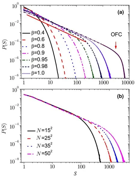
Fig.3 (Color online)Avalanche size distribution with open boundary conditions for(a)different the value of the parameter β with the system size N=352.Different curves correspond to β=0.40,0.60,0.80,0.90,0.95,and 1.0,from left to right.For comparison purposes,the original OFC model of α=0.25 is shown in the direction of the arrow.(b)Distribution of earthquake size for the different system size with β=1.0.The fitted curve is shown as red solid line.

Next,we study the other case of the modi fied OFC model(Case 2).The energy of the unstable site is redistributed to its nearest neighbors randomly and keeps some energy for itself instead of reset to zero.

In Fig.3(a),we show that the earthquakes size distributionP(S)for different values of the dissipation parameterβ,in the network withN=352and with open boundary conditions.Different curves correspond toβ=0.40,0.60,0.80,0.90,0.95,and 1.0,from left to right.It is shown that the distribution of avalanche size depends on the dissipation parameterβ.We can see that there is criticality only in the conservative case.Power-law fit is shown as red solid line,the slope of the straight line isτ=1.319 19 forβ=1.0.It is like the critical exponent of the original OFC model.For comparison purposes,the original OFC model ofα=0.25 is shown in the direction of the arrow.

The result of this case and the original OFC model tend to the same in the conservative case.The only difference is that the avalanche size in the original model is bigger.This result may be closer to the actual situation,after all,every crust plate size is different.

In Fig.3(b),we show that the earthquakes size distributionP(S)for different size of the systemN,different curves correspond toN=152,252,352and 502,from left to right.Size effect is strikingly present here in Fig.3(b).AsLorβincreases,the behavior slowly converges to a power law distribution of earthquake sizesP(s)∼s−τwith an exponentτ=1.319 19.

Fig.4 (Color online)(a)Simulation result for the probability density of having an earthquake of energy E as a function of E for a dissipation parameter β with N=352 and with periodic boundary conditions.Different curves correspond to β=0.40,0.60,0.80,0.90,0.95,and 0.98,from left to right.The fitted curve is shown as red solid line.(b)Distribution of earthquake size for the different system size with β=0.95.Different curves correspond to N=152,252,352,and 502.

Now we plot the distribution of earthquake size for different values ofβwith periodic boundary conditions.As shown in Fig.4(a),we noticed that the model transits from non-SOC to SOC behavior with the increase of the dissipation parameterβ.Power-law fit is shown as red solid line,the slope of the straights line isτ=1.427 78 forN=352andβ=0.98.Similarly,the largest size of avalanche is 108much larger than normal 103forβ=1.0.

As shown in Fig.4(b),the simulation results of avalanche size distribution in systems with dissipation parameterβ=0.95 and network sizeN=152,252,352,and 502,respectively.Although system sizes range from 152to 502,the change of the largest size of avalanche is very small.Some impact has produced on the distribution of avalanche size for the different system sizeN.We can see that size effect is exhibited but not particularly strong in Fig.4(b).We find that,asLorβincreases,the behavior slowly converges to a power law distribution of earthquake sizesP(s)∼s−τwith an exponentτ=1.427 78.

4 Conclusions

In summary,we have made an extensive numerical study of a modi fied anisotropic model proposed by Olami,Feder,and Christensen to describe earthquake behavior.The toppling rule is different with that of the OFC model.Two situations were considered in this paper.One case is that the energy of the unstable site is redistributed to its nearest neighbors randomly not averagely and keeps itself to zero.The other case is that the energy of the unstable site is redistributed to its nearest neighbors randomly and keeps some energy for itself instead of reset to zero.Different boundary conditions were considered as well.By analyzing the distribution of earthquake sizes,we found that both above cases can exhibit self-organized criticality only in the conservative case or the approximate conservative case.Some evidence indicated that the critical exponent of both above situations and the original OFC model tend to the same result in the conservative case.The only difference is that the avalanche size in the original model is bigger.It is different from the result of original OFC model.The original OFC model exhibits SOC behavior for a wide range ofαvalues and the exponentτdepend onα.This result may be closer to the real world,after all,every crust plate size is different.

[1]P.Bak,C.Tang,and K.Wiesenfeld,Phys.Rev.Lett.59(1987)381.

[2]C.Haldeman and J.M.Beggs,Phys.Rev.Lett.94(2005)058101.

[3]S.J.Wang and C.Zhou,New J.Phys.14(2012)023005.

[4]D.Plenz and H.G.Schuster,Criticality in Neural Systems,Wiley,New York(2014).

[5]S.J.Wang,G.Ouyang,J.Guang,et al.,Phys.Rev.Lett.116(2016)018101.

[6]A.Sornette and D.Sornette,Europhys.Lett.9(1989)197.

[7]B.Gutenberg and C.F.Richter,Ann.Geo fis.9(1956)1.

[8]Z.Olami,H.J.S.Feder,and K.Christensen,Phys.Rev.Lett.68(1992)1244.

[9]W.Klein and J.Rundle,Phys.Rev.Lett.71(1993)1288.

[10]K.Christensen,Phys.Rev.Lett.71(1993)1289.

[11]J.X.Carvalho and C.P.C.Prado,Phys.Rev.Lett.84(2000)4006.

[12]J.X.Carvalho and C.P.C.Prado,Phys.Rev.Lett.87(2001)039802.

[13]K.Christensen,D.Hamon,H.J.Jensen,and S.Lise,Phys.Rev.Lett.87(2001)039801.

[14]S.Lise and H.J.Jensen,Phys.Rev.Lett.76(1996)2326.

[15]M.L.Chabanol and V.Hakim,Phys.Rev.E 56(1997)R2343.

[16]H.M.Broker and P.Grassberger,Phys.Rev.E 56(1997)3944.

[17]O.Kinouchi,S.T.R.Pinho,and C.P.C.Prado,Phys.Rev.E 58(1998)3997.

[18]S.Lise and M.Paczuski,Phys.Rev.Lett.88(2002)228301.

[19]F.Caruso,V.Latora,A.Pluchino,et al.,Eur.Phys.J.B 50(2006)243.

[20]F.Caruso,V.Latora,and A.Rapisarda,Complexity,Metastability and Nonextensivity,World Scienti fic,Singapore(2005)355.

[21]N.Masuda,H.Miwa,and N.Konno,Phys.Rev.E 71(2005)036108.

[22]A.F.Rozenfeld,R.Cohen,D.ben Avraham,and S.Havlin,Phys.Rev.Lett.89(2002)218701.

[23]Min Lin,Xiao-Wei Zhao,and Tian-Lun Chen,Commun.Theor.Phys.41(2004)557.

[24]Min Lin,Gang Wang,and Tian-Lun Chen,Commun.Theor.Phys.46(2006)1011.

[25]P.Rattana,L.Berthouze,and I.Z.Kiss,Phys.Rev.E 90(2014)052806.

[26]R.Dominguez,K.Tiampo,C.A.Serino,and W.Klein,Phys.Rev.E 87(2013)022809.

[27]D.Markovic and C.Gros,Phys.Rep.536(2014)41.

[28]L.De Arcangelis,C.Godano,J.R.Grasso,and E.Lippiello,Phys.Rep.628(2016)1.

[29]A.A.Perkins,J.Galeano,and J.M.Pastor,Phys.Rev.E 94(2016)052304.

[30]Duan-Ming Zhang,Fan Sun,et al.,Commun.Theor.Phys.45(2006)293.

[31]Duan-Ming Zhang,Fan Sun,et al.,Commun.Theor.Phys.46(2006)261.

[32]Fan Sun and Duan-Ming Zhang,Commun.Theor.Phys.50(2008)417.

[33]N.Mousseau,Phys.Rev.Lett.77(1996)968.

[34]I.M.Jánosi and J.Kert´esz,Physica(Amsterdam)200A(1993)179.

[35]H.Ceva,Phys.Rev.E 52(1995)154.

[36]S.Lise and M.Paczuski,Phys.Rev.E 63(2001)036111.

[37]J.E.S.Socolar,G.Grinstein,and C.Jayaprakash,Phys.Rev.E 47(1993)2366.

[38]P.Grassberger,Phys.Rev.E 49(1994)2436.

[39]A.A.Middleton and C.Tang,Phys.Rev.Lett.74(1995)742.