Luis Fernndo Contrers,Edwin T.Brown,Mrc Ruest

aThe University of Queensland,St Lucia Campus,Brisbane,QLD 4072,Australia

bGolder Associates Pty.Ltd.,Brisbane,Australia

1.Introduction

One of the major difficulties encountered by the rock engineer is dealing with the uncertainties present in every aspect of the geotechnical design process.Uncertainty is associated with natural variation of properties,and the imprecision and unpredictability caused by the lack of sufficient information on parameters or models(Baecher and Christian,2003).Design strategies to deal with the problems associated with uncertainty include conservative design options with large factors of safety,which can be adjusted during the implementation phase based on observations of performance,and the use of probabilistic methods that attempt to measure and account for uncertainty in the design(Christian,2004).

The probabilistic method commonly used to treat uncertainty in rock mechanics design belongs to the so-called frequentist approach,but this methodology has some drawbacks(VanderPlas,2014).First,the approach lacks a formal framework to incorporate subjective information such as engineering judgement.Second,it has limitations in providing a proper measure of the confidence of parameters inferred from data.The Bayesian approach provides an alternative route to the conventional probabilistic methods used in geotechnical design;some examples are presented by Miranda et al.(2009),Zhang et al.(2009,2012),Brown (2012),Bozorgzadeh and Harrison(2014),Feng and Jimenez(2015)and Wang et al.(2016).The approach is based on a particular interpretation of probability and offers an adequate framework for the treatment of uncertainty in geotechnical design.

Probabilistic data analysis using the Bayesian approach involves numerical procedures to estimate parameters from posterior probability distributions.These distributions are the result of combining prior information with available data through Bayes’equation(Kruschke,2015).The posterior distributions are often complex,multidimensional functions whose analysis requires the use of a class of methods called Markov chain Monte Carlo(MCMC)(Robert and Casella,2011).These methods are used to draw representative samples of the parameters investigated,providing information on their best estimate values,variability and correlations.The under standing of the concepts behind various algorithms used to perform MCMC analysis is important to properly assess the quality of results.However,the analyst does not have to develop the software in order to use the method.There are already elaborated open source packages in various programming languages(Foreman-Mackey et al.,2013;Smith,2014;Vincent,2014) developed by computer scientists and related specialists,which have been tested extensively by these communities.These packages can be easily incorporated into ad-hoc codes for different modelling applications.

This paper presents initially the concepts of geotechnical uncertainty and provides a contrast between the frequentist and Bayesian approaches to quantify uncertainty.The description of the Bayesian approach with reference to the case of the inference of parameters is used to highlight the advantages of this methodology over the frequentist approach.The Bayesian methodology is applied to estimating the intact rock strength parametersσciandmiof the Hoek-Brown strength criterion(σciis the UCS of intact rock,andmiis a constant of the intact rock material),through the analysis of data from compression and tension tests.Two data set examples are presented to compare the Bayesian approach with the nonlinear least squares(NLLS)regression method representing the frequentist approach.The results of these example cases are used to discuss different aspects of the analysis,including the advantages of evaluating errors with a Student’st-distribution to handle outliers,the implications of using absolute and relative residuals,and the measure of the quality of the fitting results.The second example is used to emphasise the advantages of the uncertainty quantification with the scatter plots and bands of fitted envelopes of the Bayesian approach,in contrast to the use of confidence and prediction intervals in the frequentist method.Finally,the versatility of the Bayesian method is illustrated with two situations that require the model to be extended to include additional parameters for inference.The first case corresponds to the consideration of the Hoek-Brown parameter,a,as a free variable so that the fitting in the triaxial compression region is not constrained by that obtained in the tensile and uniaxial compression regions based on a two parameter model.The second case is the inclusion of the uncertainty in the conversion from Brazilian tensile strength(BTS)to direct tensile strength(DTS)into the overall uncertainty evaluation of the intact rock strength.

The distributions ofσciandmiresulting from the Bayesian analysis can be used as inputs for the analysis of reliability of geotechnical structures such as slopes and tunnels.The first-order reliability method(FORM)is the most common technique used for this purpose(Low and Tang,2007;Lü and Low,2011;Goh and Zhang,2012;Zhang and Goh,2012;Low,2014;Liu and Low,2017).The FORM typically considers predefined probability distributions to represent the variability of uncertain parameters and a limit state surface(LSS)defining the condition of failure of the structure.The LSS is derived from a performance function that may be available in explicit form,or alternatively,could be approximated with a response surface for complex models.

The purpose of this paper is to explain the essential differences between frequentist and Bayesian statistics in quantifying the inevitable uncertainty in experimentally determined rock mechanics parameters.While the paper uses the parameters in the Hoek-Brown peak strength criterion for intact rock material for illustration purposes,it does not explore the relationships between those parameters or their physical meanings.

2.Uncertainty in geotechnical design

The geotechnical design process implies the existence of a geotechnical model.This model is understood as the collection of elements representing different aspects of a geotechnical environment(i.e.geology,rock strength,structural features,etc.).These components include models and data used to calibrate those models by adjusting certain parameters of interest.For example,the intact rock strength can be represented by the Hoek-Brown criterion defined by theσciandmiparameters(Hoek and Brown,1997).The values of these parameters are defined through regression analysis of data from compression and tension tests on intact rock specimens.The quantification of the uncertainty of the parameters representing particular aspects of the geotechnical model is of interest to the analyst using this information for design purposes in order to assess the reliability of the system analysed.

2.1.Types of uncertainty

Uncertainty is associated with various concepts such as unpredictability,imprecision and variability.At a basic level,it can be categorised into aleatory or epistemic uncertainty.Aleatory uncertainty is associated with random variations,present in natural variability,occurring in the world or having external character,whereas epistemic uncertainty is associated with the unknown,derived from lack of knowledge,occurring in the mind or having an internal character,as discussed by Baecher and Christian(2003).Therefore,epistemic uncertainty can be reduced with the collection of additional data or by refining models based on a better understanding of the entities represented.On the other hand,natural variation cannot be reduced with the availability of more information that will only serve to provide a better representation of this type of uncertainty.

2.2.Sources of uncertainty in geotechnical design

Uncertainty is present in all aspects of the geotechnical design process.The sources of uncertainty include:

(1)Inherent variability of the basic properties considered as random variables(e.g.uniaxial compressive strength(UCS),and DTS).

(2)Measurement errors of the properties.

(3)Estimation of the statistical parameters used to represent the variables(i.e.mean,standard deviation,etc.).

(4)Approximations in the definition of sub-models to estimate derived variables(e.g.Hoek-Brown parametersσciandmiestimated from UCS,BTS and triaxial compressive strength(TCS)testing;geological strength index(GSI)estimated from structure and discontinuity condition descriptors).

A large part of the uncertainty present in the geotechnical design process corresponds to epistemic uncertainty that would be susceptible to reduction with increased data collection.However,this is often difficult to be achieved in practice because of the constraints typically operating during the site investigation stage.

2.3.Quantification of uncertainty

Uncertainties may be quantified as probabilities,which in turn can be interpreted as frequencies in a series of similar trials,or as degrees of belief.Some aspects of geotechnical engineering can be treated as random entities represented by relative frequencies while others may correspond to unique unknown states of nature,better considered as degrees of belief.An example of the former is a material property evaluated with data from laboratory testing,and any form of expert opinion represents the latter(e.g.a geological section that is constructed from site investigation data).Baecher and Christian(2003)provided a detailed discussion on the topics of duality in the interpretation of uncertainty and of probability in geotechnical engineering.They indicated that both types of probabilities are present in risk and reliability analyses,and pointed out that the separation between them is a modelling artefact rather than an immutable property of nature.

3.Probabilistic methods to treat uncertainty

Two alternative interpretations of probability provide the bases of the frequentist(classical)and Bayesian approaches of statistical analysis.The conventional approach for dealing with uncertainty in geotechnical design is based on classical statistics.In this case,data are collected and used as the only element to infer parameters and models.It will be argued that Bayesian statistical methods are a better option for treating uncertainty in geotechnical design,because they provide a formal framework for combining hard data,which are typically scarce,with other sources of information that may be available,including expert judgment.

3.1.The frequentist approach of statistical analysis

The frequentist approach of statistical analysis is based on the interpretation of probability as frequencies of outcomes of random trials repeated many times.The trials are the essence of the random sampling process central to the approach.The objective of the analysis is to infer the characteristics of a hypothesis or model from the relevant data collected randomly.The process involves the estimation of values of parameters that are assumed to be unknown,fixed quantities,whereas data are considered to be a set of random variables.This framework allows the definition of point estimates and errors of the parameters investigated that are data set-dependent.Common techniques of data analysis within the frequentist approach include maximum likelihood estimation,confidence intervals(CIs)analysis and null hypothesis significance testing.The first is a method used for the estimation of point estimates of parameters.The second provides ranges used to assess the spread of point estimates in recurring sampling.The third is a procedure used to define whether a particular value of a parameter can be accepted or rejected based on the agreement with the trend suggested by data.Frequentist statistical methods are used by default in many areas of engineering design and in many cases without full appreciation of the implications of their conceptual basis.Only recently the Bayesian approach becomes a popular alternative in geotechnical design(Miranda et al.,2009;Zhang et al.,2009,2012;Brown,2012;Bozorgzadeh and Harrison,2014;Feng and Jimenez,2015;Wang et al.,2016),as it is based on a conceptual framework suited for the treatment of geotechnical uncertainty.

3.2.The Bayesian approach of statistical analysis

The Bayesian approach of statistical analysis is based on the interpretation of probability as degrees of belief.The inference process with this approach combines existing information on the model or hypothesis to be examined,known as priors,with the data from sampling using Bayes’rule.An important aspect of the Bayesian approach is that the sought parameters of the models or hypothesis being examined are considered to be random variables,whereas data are assumed to be fixed known quantities.The results of Bayesian analyses are probability distributions known as posteriors.

Bayes’rule was named after Thomas Bayes,whose work on this topic was published in 1763,two years after his death(Bayes,1763).Bayes’rule can be derived from basic definitions of conditional probability and allows the calculation of the probability of the hypothesis given the datap(H|D),from the probabilities of the data given the hypothesisp(D|H),the hypothesisp(H),and the datap(D).

The general form of Bayes’equation is

The Bayes’equation is used to update knowledge of a hypothesis or model from observations represented by the data.The updating process is done by quantifying the uncertainties of the model parameters when there is no information on the characteristics of their distributions.Detailed information on Bayesian analysis at introductory to advanced levels can be found in several texts(e.g.Gregory,2005;Sivia and Skilling,2006;Gelman et al.,2013;Stone,2013;Kruschke,2015).

3.2.1.The posterior distribution

The “posterior”is a probability distribution that balances the knowledge provided by the prior information and the data.If sufficient data are available,data will drive the result.If the data component is weak,prior knowledge will have a strong effect.All of this is handled within the Bayesian approach in a rational manner,without external manipulation.The posterior is the answer of interest to the data analyst,but this distribution is typically complex and its evaluation requires the use of special numerical techniques.

3.2.2.The likelihood function

The “likelihood”function defines the probability of obtaining the observations included in the data set given the model or hypothesis under examination.The likelihood is the answer given by classical statistical methods.Fig.1 adapted from Kruschke(2015)shows an example of the calculation of the likelihood of a data set of three points,D={85,100,115},assuming that its variability is represented by a normal distribution with mean,μ,and standard deviation,σ.The likelihood is calculated for three values ofμ (87.8,100,112)shown in the column plots and three values ofσ(7.35,12.2,18.4)shown in the row plots.The probability of an individual point is represented by the vertical dotted line over the point and the probability of the data setp(D|μ,σ)is the product of the three individual probabilities as expressed by the likelihood function.As expected,the maximum likelihood result(7.71 10-6)corresponds to the mean(μ =100)and standard deviation(σ =12.2)of the data points.

3.2.3.The prior distribution

Fig.1.Example of the calculation of the likelihood of a data set of three points,assuming a normal distribution and testing different values of mean,μ,and standard deviation,σ.Columns show different values ofμ and rows show different values ofσ.The middle plot shows the maximum likelihood result(adapted from Kruschke,2015).

The “prior”represents the initial knowledge,or lack of it,in the hypothesis,and therefore can be either informative or vague.Informative priors can be any type of distribution that represents adequately the existing knowledge of the model or parameter being examined.However,the usual situation is that there is little information available,so the goal becomes to encode this lack of knowledge in a non-informative or vague probability distribution to avoid constraining the results.This is done with distributions derived by applying the maximum entropy principle(Jaynes,1957).In this case,entropy refers to disorder or randomness in the information,and has similarity with the concept of entropy in physical systems.The uniform distribution is a common maximum entropy distribution and corresponds to the situation in which only the limits of the parameter are known.The selection of the prior is an important step in Bayesian data analysis.The prior could add valuable available information to the posterior if selected adequately,or it could bias the results if it over-constrains the data.

3.2.4.The evidence function

The “evidence”part in the denominator of Bayes’equation is normally treated as a normalisation factor so that the posterior integrates to one.It is calculated as the integral over the whole parameter space of the numerator,i.e.as the product of the likelihood function and the prior distribution.The posterior distribution does not need to be normalised when the purpose of the Bayesian analysis is the inference of the uncertain parameters using a numerical approach such as the MCMC.Therefore,the calculation of the typically complex integral in the denominator of the Bayes’equation can be omitted.The denominator is required when the objective of the analysis is the comparison of two alternative models,which is done through the calculation of the Bayes factor.

3.3.Contrast between the frequentist and Bayesian approaches

The more relevant points of contrast between the frequentist and Bayesian approaches are summarised in Table 1(Contreras and Ruest,2016).The second aspect constitutes one of the more important advantages of the Bayesian approach as it addresses the question of interest to the geotechnical engineer.This aspect is also at the base of misunderstanding about the type of answer that classical statistical methods provide.The results of Bayesian analyses are richer and more informative than the conventional point estimates and error measurements given by the frequentist approach.The conceptual framework of the Bayesian approach is better suited to the task of the inference of parameters to investigate models.

3.4.Example to contrast the results from the two approaches

A consequence of the different interpretations of probability is the contrasting assumptions regarding data and parameters made by the approaches.This,in turn,affects how the boundaries of model parameters are determined.In the frequentist approach,CIsfrom data are used to define meaningful parameter boundaries,whereas in the Bayesian approach this is done with credible regions of the posterior distribution.

Table 1Key aspects of contrast between the frequentist(classical)and Bayesian approaches to statistical analysis(adapted from Contreras and Ruest,2016).

The CI is defined by upper and lower bound values above and below the mean of a data sample,and is associated with good estimates of the unknown population parameter investigated.The CI is calculated from a particular sample with its width depending on the number of data points in the sample,and the chosen level of confidence for the estimation.For this reason,this result is commonly used as a measure of confidence of parameter estimates without having a full understanding of its meaning.A CI is specific to a data set and its confidence level only has meaning in repeated sampling.For example,if the 95%CI for the mean UCS of a particular rock type is constructed,it either includes the true UCS value or does not,but it is not possible to know the situation for that particular CI.The 95%confidence means that if the sampling process is repeated numerous times,and CIs are calculated for those various samples,95%of the sample sets will have CIs containing the true UCS value.However,because the true value is an unknown fixed parameter in the frequentist framework,it is not possible to identify the sample sets containing the true UCS.The uncertainty regarding the true UCS value remains.

Fig.2 shows an example of repeated sampling that provides an appreciation of the meaning of the CI in the frequentist approach.The values could represent UCS results for a particular rock type,but the data were randomly generated to illustrate the point.A total of 100 data sets of 15 values each were sampled from a normal distribution with a mean of 120 MPa and a standard deviation of 30 MPa that represent the unknown fixed parameters of the population.Each data set has its own mean and standard deviation and the bars in Fig.2 correspond to the 95%CIs of the mean.However,for this particular group of data sets,91 of the intervals contain the true mean.A larger number of data sets would be required to obtain a better approximation of the 95%level used for the construction of the intervals.Nevertheless,the important point with this example is that in terms of each individual data set,there is no probability associated with the inclusion of the true mean.The interval either includes it or does not.In a real case,there would be only one data set and it would not be possible to estimate the true value.

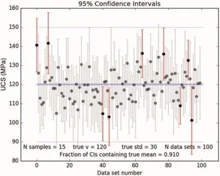
Fig.2.Frequentist interpretation of CIs for randomly generated UCS data sets of 15 values with a mean of 120 MPa and a standard deviation of 30 MPa.

In the Bayesian approach,the situation is different because the unknown parameter being investigated is considered to be a random variable that is updated for every new data set.The posterior probability distribution resulting from the Bayesian updating process is used to define the highest density interval with a particular level of precision.This interval defines the bounds of the credible region for the estimation of the parameter.In many simple situations,the results from both approaches coincide,but the meanings of the results are different.The Bayesian result has a meaning consistent with the answer that is normally sought by the analyst,whereas the frequentist result responds to a different question that is of less interest to the analyst.

Fig.3 compares the frequentist 95%CI for data set 27 in Fig.2 with the credible interval corresponding to the 95%high-density interval(HDI)of the posterior distribution from a Bayesian estimation of the mean.The posterior distribution is calculated for the same data set,assuming a uniform prior distribution,which is considered to be a non-informative prior in this case.The results show that the prior does not affect the likelihood of the data,yielding a result that appears to coincide with the frequentist result,although with a different meaning.In this case,the Bayesian interval indicates a range for the sought mean with a 95%credibility.This is possible because,in the Bayesian framework,the parameter investigated is not fixed but changes as new data become available.The frequentist result corresponds to a point estimate of the mean and a measure of the error represented by the width of the CI,whereas the Bayesian result provides a full probability distribution for the mean based on the data used.

4.Bayesian inference of uncertain parameters

Fig.3.Comparison between the frequentist(left)and Bayesian(right)results for the inference of the mean UCS of data set 27 in Fig.2.

Fig.4.Conceptual representation of the Bayesian model for inference of parameters.

Three elements are required for the construction of a Bayesian model for the inference of parameters.Fig.4 shows a conceptual representation of this model.First,there must be a model in the form of a mathematical function that represents the performance of a particular system of interest.This model includes predictor variable,x,and the parameters for inference,θ.Second,there must be data that normally correspond to measurements of actual performance of the system,yactual,to compare with the model predictions,ymodel.Third,there is the prior knowledge available on the parameters;this means any type of information,for example valid ranges or credible values.These elements are combined in a probabilistic function that contains the set of uncertain parameters for inference,θ1to θk.This function effectively corresponds to a posterior probability distribution using the Bayes’equation and gives probability values,p,for particular sets of uncertain parameters,θ.The objective of the analysis is to define the sets ofθ that produce the largestpvalues.In other words,the objective is to define the most probable parameter values.

4.1.Generic formulation of the model for Bayesian inference of parameters

Zhang et al.(2009,2012)described the concepts of characterisation of geotechnical model uncertainty in a Bayesian framework.The following presentation uses some elements of that account but it is adapted to fit the case of the intact rock strength model discussed in Section 5.

A model can be represented by a functionfused to predict a system response,ymodel:

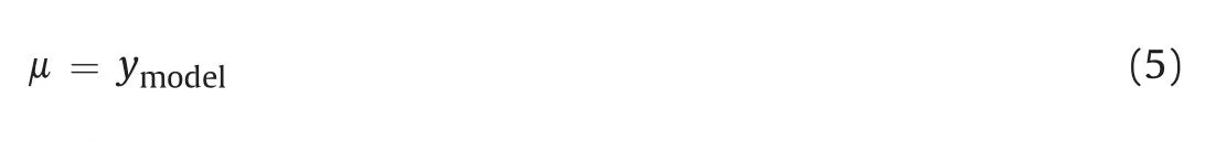
The function depends onθand r,which are vectors with the uncertain and certain parameters of the model,respectively.The certain parameters include the predictor variablesx,which are those variables used to define the predicted variabley,whose behaviour is targeted with the model.If there are measurements of the actual system response,yactual,then it is possible to define the error,ε,that accounts for model uncertainty:

The error,ε,is assumed to have a Gaussian(normal)distribution,with mean,μ,and standard deviation,σ.Alternatively,at-distribution can be used to represent the variability of ε and to give improved handling of any outliers.In this case,an additional parameter called normality,ν,is required,which controls the weight of the tails of the distribution.Thet-distribution coincides with the normal distribution whenνis equal to or greater than 30.For simplicity,a normal distribution is considered in the description of the method that follows.

The errors are assumed to be normally distributed around the model prediction,so that we have

and

In this case,the standard deviation of the errors,σ,is the only so called nuisance parameter that needs to be inferred together with the model parameters of interest in the vector,θ.

The Bayesian approach can be used to evaluate the posterior probabilityp(θ,σ|D)of the uncertain parameters used in the model given the data D on the actual performance of the system modelled:

Eq.(7)is an extended version of the Bayes’equation shown in Eq.(1).Vague priors are used if there is little information on the values of the uncertain parameters.In this case,the prior termp(θ,σ)is defined with uniform distributions forσ and thekuncertain parameters inθ:

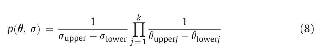
The subscripts in this equation refer to upper and lower values defining credible ranges of the uncertain parameters.The likelihood termp(D|θ,σ)is defined using a normal distribution to reflect the Gaussian variability of the errors,ε.The calculation is carried out for thenmeasurements of the system response:

The likelihood term is defined as the probability of the data given the uncertain parameters,but it can also be presented as the likelihood of the parameters given the data:

The denominator in Eq.(7)is calculated as the integral of the numerator across the whole parameter space.This is the normalisation term not required for inference of parameters with a MCMC procedure.This term is required for the calculation of the Bayes factor used for model comparison.The formula for the posterior distribution in Eq.(7)can become a complex expression if the model in Eq.(3)itself is a complex formula with many uncertain parameters.An efficient way of evaluating this function is by obtaining representative samples of the parameter values using the MCMC procedure.

4.2.The Markov chain Monte Carlo(MCMC)method

The MCMC method is a procedure for sampling a probability distribution based on the selection of representative samples according to a random process called a Markov chain.In a Markov chain,every new step of the process depends on the current state and is completely independent of previous states(Kruschke,2015).One of the main applications of the MCMC method is the evaluation of complex probability distribution functions of many dimensions such as those encountered in the posterior or likelihood functions of Bayesian data analysis.The Markovchain,also called the random walk,in spite of being a random process,will always mimic the target distribution in the long run.The increased use of MCMC methods during the last 15 years is related to advances in computer hardware and numerical algorithms facilitating the use of these methods.There are numerous books and papers devoted to the subject of the MCMC method.For example,Diaconis(2009)provided some examples of formerly intractable problems that can now be solved using this technique.Robert and Casella(2011)presented a brief history of MCMC and provided a comprehensive treatment of MCMC techniques(Robert and Casella,2004).

Several algorithms are used toimplement a MCMC process,with the Metropolis,Gibbs and Hamiltonian algorithms being among the more commonly used ones(Kruschke,2015).In general,all the algorithms share the following basic steps:

(1)Start with an initial guess of the set of parameters to sample.

(2)Evaluate a random jump of the set of parameters from their current values.

(3)Evaluate the probabilities of the proposed and current sets of values with the target distribution.

(4)Use the ratio between the probabilities of the proposed and current sets of values to define a criterion of acceptance of the jump.The criterion should favour moves towards the regions of higher probability,but should not eliminate the possibility of moves towards the regions of lower probability.

(5)Apply the acceptance criterion to update or retain the current values and repeat the process from step 2 until a sufficient number of sets of values(samples)are defined.

One advantage of this procedure is that it works even if the target function is not normalised to conform to the definition of a probability distribution.

4.3.Assessment of the quality of the MCMC analysis results

An MCMC sample should be representative of the posterior distribution,should have sufficient size to ensure the accuracy of estimates,and should be generated efficiently(Kruschke,2015).In general,the implementation of an MCMC process requires some adjustments to achieve a stable solution in the form of representative independent samples from the parameters.It is common to discard a portion of the early steps of the chain,known as the burnin process,while the sampling sequence evolves into a stable process.Diagnostic checks carried out on graphs produced with the results of the analysis serve to assess the quality of results.Some algorithms have heuristic rules on the acceptance rate of the steps of the chain to ensure that the samples are independent and representative of the posterior distribution.For example,for the affine-invariant assemble sampler used for the examples discussed in this paper,the recommendation is to have a rate of between 20%and 50%(Foreman-Mackey et al.,2013).

4.4.Software for MCMC analysis

Although it is important to understand the concepts behind the various algorithms used for the MCMC analysis to properly assess the quality of the results,the analyst does not have to programme these algorithms.There are already elaborated open source packages in various programming languages developed by computer scientists and related specialists that can be easily incorporated into ad-hoc code.Vincent(2014)listed some currently available popular packages for MCMC.The models described in this paper were coded in the Pythonprogramming language(Python Software Foundation,2001)and the posterior distributions were sampled with the ‘emcee’Python package developed by Foreman-Mackey et al.(2013).The software includes an algorithm known as the affine-invariant ensemble sampler characterised by the use of multiple chains running simultaneously to explore the domain of the function.The software is developed and used by the astrophysics community with complex multidimensional models that exceed the expected complexity and dimensionality of the models normally used for geotechnical analysis.

5.Bayesian inference of intact rock strength parameters

5.1.Description of the method

The Bayesian estimation of intact rock peak strength parameters is based on the Hoek-Brown strength criterion(Hoek and Brown,1997)defined by the following equation:

where σ1and σ3are the major and minor principal stresses,respectively.σciandmiare the parameters investigated with the analysis.Using this criterion,the intact tensile strength,σt,is given by

The data correspond to the results of TCS and UCS tests and DTS estimates made from BTS test results.These results correspond to measurements of one of the principal stresses at failure for particular values of the other principal stress.For example,the results of TCS and UCS tests provide measurements of the major principal stress,σ1,at failure for fixed values of the minor principal stress,σ3,with compression taken as positive.The DTS values correspond to σ3measurements at failure when σ1is zero.The estimation of DTS is normally based on indirect measurements made using the BTS test.Perras and Diederichs(2014)found good rock type-dependent correlations between DTS and BTS results with suggested correlation factors ofα=DTS/BTS of 0.9 for metamorphic rocks,0.8 for igneous rocks,and 0.7 for sedimentary rocks.

Langford and Diederichs(2013,2015)discussed the estimation of Hoek-Brown intact rock strength envelopes from laboratory test results using a frequentist approach.In their latter paper,they compared three regression methods to estimate the best-fit envelope,namely,two variants of ordinary least squares with the linearised form of the Hoek-Brown strength equation,and a nonlinear regression method with the equation in its original form.These two versions of linear regression refer to the inclusion or otherwise of the adjustment for the measurement of errors in the tensile zone.The nonlinear method includes this adjustment.Langford and Diederichs(2013,2015)considered nonlinear regression to be the preferred method of producing the best fits.In terms of uncertainty evaluation,they used the concept of prediction interval(PI)to quantify the uncertainty of data.Subsequently,they made assumptions regarding the correlation characteristics between UCS andmito fill the PIs with Hoek-Brown envelopes in order to assess the variability of these parameters.However,as will be discussed in Section 5.5,the use of PIs to assess the uncertainty of the fitted envelopes is not consistent with the standard concept of PI in the frequentist approach.

As indicated in Section 3.2,in the Bayesian approach,data are fixed whereas parameters are random.This characteristic results in a much clearer and sounder assessment of the uncertainty of the parameters.The result of the Bayesian analysis consists of probability distributions ofσciandmias well as scatter plots of sampled values providing information on their correlation characteristics.This information is used to produce the band of plausible failure envelopes reflecting the uncertainty of the intact rock strength.

Fig.5.Measurement of errors in the tensile and compressive strength regions with a tdistribution to handle outliers.

The Bayesian analysis in this paper is compared with the NLLS regression method used by Langford and Diederichs(2015).Both methods consider the correct direction of measurement of errors,i.e.errors inσ1are calculated for UCS and TCS data,whereas errors inσ3are evaluated for DTS data.Fig.5 shows the way in which errors are measured in the Bayesian analysis.The linear regression method is not considered with the Bayesian analysis because the indirect estimation of the parameters causes some drawbacks with regard to the selection of vague priors.This is because the parameters inferred using the linear regression approach are the intercept and the slope of the Hoek-Brown linearised equation,and the vague condition of their priors is not transferred to the parameters of interest,σciandmi.

Fig.6 illustrates the structure of the Bayesian model for the robust estimation of intact rock strength parameters.The model combines the prior and the likelihood parts to define the posterior function according to Bayes’rule.The Hoek-Brown criterion represents the model whose predictions are compared with data to define errors,which are evaluated with at-distribution to construct the likelihood function.

A problem commonly met in regression analyses is the bias in the estimation of parameters caused by the presence of outliers in the data.A way to deal with this situation is to consider at-distribution to represent the spread of the data points in the direction of measurement of errors.Thet-distribution is defined by three parameters that control the central value(mean,μ),the width(scale,σ)and the weight of the tails(normality,ν).The possibility to set heavy tails with this distribution allows outliers to be accommodated without shifting the mean.This point is illustrated in Fig.7(taken from Kruschke,2015)where the advantage of thetdistribution over the normal distribution is highlighted.The use of thet-distribution for modelling errors makes the method robust in the true statistical sense.

The Bayesian model considers prior distributions of four parameters-the rock mechanics parameters,σciandmi,modelled with uniform distributions,and the scale,σ,and normality,ν,parameters of thet-distribution modelled with uniform and exponential distributions,respectively,as shown in Fig.6.The uniform distributions are defined within valid ranges of the parameters determined by lower and upper bound values.The vague priors of the rock mechanics parameters are intended to limit their variations to plausible values without constraining the estimation within those limits.The ranges used for the examples in this paper are 10-500 MPa forσciand 1-50 formi.

The range for the parameterσis based on the characteristics of the data set with lower and upper values defined as the standard deviation of data in theyaxis(stdev.σ1)divided and multiplied by 100,respectively.The prior for the parameterνis an exponential distribution with mean 1/29 because the majority of the changes of thet-distribution occur for values between 1 and 30.Whenνis greater than 30,thet-distribution coincides with the normal distribution.In this way,the full range of tail shapes of thet-distribution has similar chances of being selected.The one added to the value sampled from the distribution is intended to convert the range of the exponential distribution from 0 to infinity to the valid range ofνfrom 1 to infinity.

The details of the definition of the posterior distribution function for the conditions of analysis presented in this paper are included in Appendix.The posterior is a cumbersome four-dimensional function that is better evaluated by sampling the parameters with an MCMC algorithm.The model was implemented in the Python programming language,using the MCMC sampler “emcee”.

Finally,in this account of the methods of analysis to be used in the illustrative examples to follow,it is important to offer a qualification about the UCS data used in the examples.It has been established that the value of the UCS parameter,σci,used in fitting the Hoek-Brown criterion to the peak TCS data for intact rock,should be the value obtained from the intercept of the peak strength curve with theσ3=0 axis(Hoek and Brown,1997;Bewick et al.,2015;Kaiser et al.,2015).This value may correspond to the results of well-conducted UCS tests in which shear failure occurs,but is usually higher than the UCS value obtained from tests in which splitting failure occurs.It should be noted that in the data analysed here,no attempt has been made to differentiate between samples showing these different modes of failure.

Fig.6.Conceptual basis of the Bayesian model for the robust estimation of the Hoek-Brown intact rock strength parameters,σciand mi.

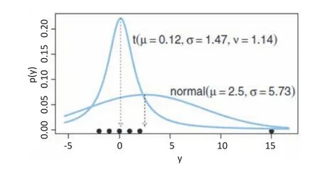
Fig.7.Illustration of the advantage of the t-distribution over the normal distribution to accommodate outliers in robust statistical inference(Kruschke,2015).

5.2.Example of fitting data with outliers

The methodology is illustrated using a “typical”intact rock strength data set of 60 points(15 UCS,15 DTS and 30 TCS),including a few outliers,which was generated using random numbers between pre-defined limits.The analysis was carried out with a reduced data set of 31 points(8 UCS,8 DTS and 15 TCS)without outliers,and with the complete data set of 60 points,in order to highlight the effect of the outliers.Fig.8 shows the data points together with the fitted envelopes using the NLLS regression method and the Bayesian approach.The NLLS method is based on the numerical estimation of the set of parameters that minimises the squared residuals function.The Bayesian method is denoted as MCMC_S in Fig.8 to indicate that the MCMC sampling is done on a posterior function using at-distribution to model the errors.The two methods shown in Fig.8 consider the actual(absolute)residuals for the calculation of errors.The results of the analyses are similar for the case with 31 data points but differ for the case of 60 data points with a marked effect from the outliers on the NLLS envelope.On the other hand,the Bayesian result appears to be less affected by the outliers,demonstrating the robustness of the method.

One aspect of the data set that has an impact on the fitting result is the fact that the errors in the tensile region are one order of magnitude smaller than the errors in the compressive region.For example,the case without outliers in Fig.8 shows that the range of tensile strength values is about 5 MPa whereas the compressive strength values are 10 times more variable.One way of accounting for this imbalance with the Bayesian model would be to set up separatet-distributions to model tensile and compressive errors.This adjustment would imply the addition of two uncertain variables to be inferred.However,a simpler alternative also available to the frequentist method is the normalisation of errors with the respective model values.The relative residuals calculated in this way would have similar orders of magnitude in the tensile and compressive regions.

Fig.8.Comparison of fitted Hoek-Brown failure envelopes with nonlinear least squares(NLLS)and Bayesian sampling(MCMC_S)methods,considering absolute residuals(abs).Data sets of 31 points without outliers(left)and 60 points with outliers(right)were used.

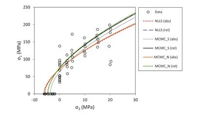
Fig.9.Comparison of fitted Hoek-Brown failure envelopes with nonlinear least squares(NLLS)and Bayesian sampling(MCMC_S and MCMC_N)methods,considering absolute(abs)and relative(rel)residuals and the data set of 60 points.

Fig.9 shows the data points for the case of 60 test results and the six fitted envelopes using three methods of analysis with absolute and relative residuals.The methods include the NLLS,the Bayesian sampling of a posterior function based on at-distribution for the errors(MCMC_S),and the Bayesian sampling of a simpler function using a normal distribution to model the errors(MCMC_N).The reason for using a model with the normal instead of thet-distribution is to appreciate the real effect that the use of relative errors has on the bias caused by the outliers.

The results in Fig.9 show coincidence of the envelopes defined by the three methods when the errors are normalised(relative residuals).The results of the analysis with absolute residuals show the strong effect of the outliers on the envelopes fitted with the NLLS and the Bayesian with normal distribution methods.These results also highlight the robust effect of thet-distribution in the Bayesian model indicated by the closeness of the result to the fitted envelopes using relative residuals.

5.3.Comparison of regression methods

The quantification of the goodness of fit with the NLLS method is based on the standard error(SE),which can be calculated for absolute and relative residuals.The SE of the fitted envelopes defined with two parameters fromndata points is calculated as

The SE can also be calculated for the envelopes obtained from the Bayesian analysis.However,in this case,a more adequate indicator of the goodness of fit is the maximum likelihood value(MxL)that measures the likelihood of the estimated parameters.The MxL is calculated with the model described in Fig.6.Likelihood values correspond to the product of small probabilities of the individual data points;therefore,they are very small numbers.For this reason,the maximum likelihood estimations are normally reported as the logarithms of the values.The comparison of the maximum likelihood values to assess the effectiveness of the regression models is meaningful when the two competing models have the same numbers of parameters.If the models have different numbers of parameters,the appropriate way to compare the models is through the Bayes factorK,defined as the ratio of the evidence terms of the two competing models:

The evidence termp(D|model)corresponds to the integration of the numerator of the Bayes posterior over the parameter domains(see Eq.(7)).A model with more parameters having a greater maximum likelihood due to smaller errors is not necessarily better than a model with a lesser maximum likelihood but with fewer parameters.The Bayes factor,K,provides the appropriate measure of the relative effectiveness of the two models.

Table 2 shows a summary of the results of the six regression analyses presented in Fig.9.The table includes the main characteristics of each regression model,the estimated parameters,the SE for absolute and relative errors,and the natural logarithm of MxL for the Bayesian analysis.As expected,the minimum SEs with absolute residuals are obtained with the methods that use the absolute residuals in the calculation process,and similarly occur with the minimum SE with relative residuals.The MxL results of the four Bayesian models indicate a better fit with the models that use relative residuals as compared with the models based on absolute residuals.A proper comparison of the effectiveness of the Bayesian models is shown in Table 3 which includes the Bayes factors for all the model pairs.

A commonly used interpretation of the Bayes factor for model comparison is indicated in Table 4(Kass and Raftery,1995).According to this interpretation,the Bayes factors in Table 3 indicate very strong support of the models based on relative residuals as compared to the models that use absolute residuals.In terms of the type of distribution used to model the errors,the models based on thet-distribution and the normal distribution are effectively equivalent.However,the calculated Bayes factors are specific to the data set used for the analysis.Therefore,it is concluded that the model based on thet-distribution with relative residuals is the preferred fitting method,since it will provide a superior handling of potential outliers in any of the test results.

5.4.Additional results from the Bayesian approach

A notable feature of the Bayesian analysis is that the parameters are defined from complete probability distributions that not only provide information on the reliability of the estimates,but also indicate their correlation characteristics.In this respect,the Bayesian method can provide a complete quantification of the parameter uncertainty.

Fig.10 shows the scatter plots ofmiversusσcivalues obtained from the Bayesian analysis using the four models implemented.The graphs at the left are from the analysis with absolute residuals and those at the right are from the analysis with relative residuals.The graphs at the top correspond to the models based on thet-distribution and those at the bottom are from models using the normal distribution to evaluate the errors.The contours define the 95 and68 percentiles of sampled points and the crosses mark the mean values.The calculated coefficients of correlation(CC)are indicated in the upper right corner of each plot.The parameters show a negative correlation for the analysis with absolute residuals,which is a consequence of the difference in the order of magnitude of the errors in the tensile and compressive strengths.The normalisation of the errors causes the narrowing of the likely tensile strength,which translates to the reduction in the spread of theσciandmivalues.This effect is better appreciated in the graphs of Fig.11 showing the bands of envelopes corresponding to the 95%of sampled values for the cases of absolute and relative residuals.The results in Figs.11 and 12 confirm the benefit of normalising the errors for the regression analysis and the indifference of the results with relative residuals to the type of distribution used to evaluate these errors.

Table 3Effectiveness of Bayesian regression models based on Bayes factor comparisons.

Table 4Interpretation of Bayes factors(Kass and Raftery,1995).

Fig.12 shows the histograms of the representative samples ofσciandmidrawn from the posterior distribution,for the case of relative residuals evaluated with thet-distribution.The histograms define the ranges of credible values corresponding to the 95%HDIs and the more likely estimates represented by the mean values(σci=75 MPa andmi=15.6).

Fig.13 shows the complete set of results of the MCMC analysis for the case of relative residuals evaluated using at-distribution.The graph includes the scatter plots between all the parameters sampled from the posterior distribution as well as the histograms of those parameters.The graph shows not only the results of the parameters of interest,σciandmi,but also the nuisance parameters,σ andν,used in the model to characterise thet-distribution.The parameterνis plotted in logarithmic form to facilitate an appreciation of its variability.These plots are useful for identifying correlations and for detecting possible anomalous situations that might suggest instability of the chains or other problems with the sampling process.

The specification of the MCMC sampling process included 50 chains,also known as walkers,with 2000 steps per walker and excluding half of the steps as part of the burn-in process.Animportant diagnostic graph to verify the validity of the results is the trace plot shown in Fig.14.Trace plots show the progress of the 50 chains sampling each parameter through the total number of steps specified.They indicate that a stable process was reached in a few steps,suggesting that fewer steps may have been sufficient to sample the function.The acceptance rate of the sampling process was 0.47 which is within the limits recommended for the affine invariant assemble algorithm(Foreman-Mackey et al.,2013).

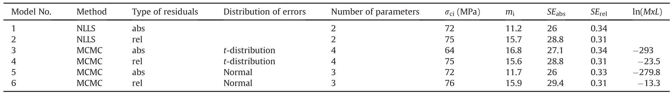
Table 2Comparison of results of fitting analysis.

Fig.10.Scatter plots of miversusσcifrom the Bayesian regression analysis with absolute(left)and relative(right)residuals.Models based on t-distribution(top)and normal distribution(bottom)were used to evaluate the errors.

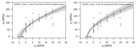
Fig.11.Fitted envelopes with bands corresponding to the 95%of sampled points from the analysis with absolute(left)and relative(right)residuals,and the model based on the tdistribution to evaluate errors.

5.5.Comparison between the uncertainty evaluations with the frequentist and Bayesian approaches-a second example

Given the merits of considering relative residuals to obtain the best estimation of the intact rock strength parameters,the focus in this section is on the quantification of the uncertainty of these parameters.The example presented in the preceding sections showed coincidence between the NLLS and Bayesian results for the analysis with relative residuals.The example also served to highlight the main features of the quantification of uncertainty of the parameters inferred with the Bayesian approach.Sections 5.5-5.7 illustrate the contrast between the uncertainty quantification with the two approaches,by analysing a data set of 166 test results on samples of a homogenous granite in Sweden.The data set includes 70 BTS,59 UCS and 37 TCS tests with confining pressures between 2 MPa and 50 MPa.The tests were carried out at the Swedish National Testing and Research Institute(SP)for the Swedish Nuclear and Fuel Waste Management Company(SKB).The data were extracted from 14 publically available data reports concerning the Oskarshamn site investigation in Sweden(Jacobsson,2004,2005,2006,2007).All of the results in the data set correspond to tests on intact rock with failure modes not affected by local defects.

Fig.12.Posterior distributions ofσciand miwith mean and 95%HDIs indicated,for the case of relative residuals evaluated with a t-distribution.

The two regression methods considered for the comparison of uncertainty quantification are the NLLS and the Bayesian sampling with the model based on at-distribution to evaluate the errors(MCMC_S).In both cases,the analyses are carried out with relative residuals.

5.6.Confidence interval(CI)and prediction interval(PI)in the frequentist approach

The conventional way of measuring the uncertainty of a parameter estimate within the frequentist approach is to construct a CI around the inferred point estimate.In this case,the parameter is non-random and unknown.The interpretation of a 95%CI is that in repeated sampling,95%of the intervals constructed around their respective point estimates will contain the true fixed but unknown value of the parameter.In the Hoek-Brown strength envelope case,the fitted envelope defined by the parametersσciandmiis the point estimate and the 95%CI is defined as follows for the compressive and tensile strength regions:

whereσtis the tensile strength for the fitted strength envelope;t2.5%，n-2is the 2.5 percentile of thet-distribution withn-2 degrees of freedom,which defines the interval that includes 95%of the area of thet-distribution with a zero mean;SEris the standard error as defined by Eq.(13)considering normalised(relative)errors;nis the number of data points;and μσ3datais the mean of the σ3datavalues.

The PIs within the frequentist approach have a different meaning and refer to the uncertainty of data values which are considered to be random variables.The interpretation of a 95%PI is that there is a 95%probability that the next data value to be observed will fall within the interval.In the Hoek-Brown strength envelope case,the fitted envelope defined by the parametersσciandmican be used to predict individual strength values.A 95%PI constructed around this envelope defines the limits where future strength observations will be with a 95%probability.The 95%PI is defined as follows for the compressive and tensile strength regions:

The PI and CI are centred on the fitted envelope,but the PI is wider than the CI,because the PI refers to the variability of individual data points,whereas the CI is associated with the variability of the whole envelope.In both cases,it is implied that there must be additional sampling for the levels of confidence to have a meaning.In the case of the PI,a future data point is required,whereas for the CI,many similar data sets need to be collected.

Fig.15 shows the data set and the results of the frequentist analysis that include the fitted envelope with the 95%CI and PI around the mean.The intervals are narrower towards the mean of theσ3data range.This effect is compounded with the widening of the interval relative to the model fit value that multiplies theSEr.Langford and Diederichs(2015)used the PI to quantify the uncertainty of the fit.However,as indicated above,within the frequentist approach,the uncertainty of the fit is measured with the CI,whereas the uncertainty of the data points is associated with the PI(Hyndman,2013).

5.7.Scatter plots and envelope bands in the Bayesian approach

Fig.16 shows the results of the fitting analysis of the data set using the Bayesian approach.In this case,the samples drawn from the posterior function with the MCMC procedure are represented in the scatter plot ofmiversusσcion the left in Fig.16.This graph indicates a positive correlation between the two parameters and provides a complete description of their uncertainty.The outer contour in the scatter plot corresponds to the 95 percentile of the sampled values and the envelopes constructed with these values define the envelope band represented in the graph on the right in Fig.16.The narrow band suggests a sharp definition of the Hoek-Brown strength envelope supported by the 166 test results in the data set.This is not a typical number of test results available in many projects.Fewer data will result in wider uncertainty bands.

Fig.13.Corner graph showing the scatter plots of pairs of all the sampled parameters and their individual histograms.

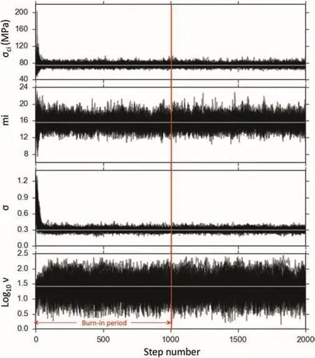
Fig.14.Trace plots of the MCMC chains for the four parameters sampled from the posterior distribution.Each plot includes the traces of the 50 walkers used for the sampling giving a total of one hundred thousand samples per parameter.The first fifty thousand steps correspond to the burn-in process and were excluded from the results.

The results shown in Figs.15 and 16 show coincidence in the estimation of the mean envelope,but highlight the differences in the evaluation of the uncertainty of the intact rock strength parameters.The frequentist approach provides intervals where the envelope or a data point may be found with a level of confidence.However,for this approach,the level of confidence only has meaning if repeated future sampling is carried out.The Bayesian method provides a representative sample of parameter values with the highest probability of occurrence based on the set of test results used in the analysis.The sampled values allow the definition of the range of credible envelopes for a particular level of confidence.The Bayesian method offers a richer and clearer evaluation of the uncertainty of the intact rock strength parameters.

Fig.15.Uncertainty quantification of the Hoek-Brown intact rock strength envelope with the frequentist approach(NLLS method with relative residuals).Fitted envelopes,95%CI reflecting the uncertainty of the mean envelope and 95%PI reflecting the uncertainty of individual data points.

Fig.16.Uncertainty quantification of the Hoek-Brown intact rock strength envelope with the Bayesian approach(model based on relative residuals with t-distribution).Scatter plot of sampled values of miversusσciwith 68 and 95 percentile contours(left).Fitted envelope and band of envelopes corresponding to the 95%of sampled parameter values(right).

5.8.Improving the fit in the triaxial region

The Hoek-Brown par ameters σciandmiinferred from the fitting analysis define the intercepts of the peak strength envelope with the tensile and uniaxial compressive strength axes.However,the fit in the triaxial region is constrained by the assumption that the parameter,a,in the generalised criterion for rock masses is 0.5 for intact rock,as indicated by the exponent in Eq.(11).The Bayesian approach provides a convenient way to assess the merits of including the parameteraas an additional uncertain variable for inference.Langford and Diederichs(2015)described the improvement of the fit with a frequentist approach when the parameterais included in the analysis.They also pointed out the practical difficulties of implementing this modification to the criterion for intact rock strength.

Fig.17.Corner plot from the analysis of the Swedish granite data set considering the Hoek-Brown parameter a as variable.The plot shows the scatter plots and histograms of the rock mechanics parameters.

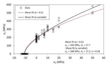
Fig.18.Comparison of the fitted envelopes from the analysis with the parameter afixed to 0.5 and for the case in which a is variable.

Fig.19.Uncertainty of the Hoek-Brown intact rock strength envelope when the parameter a is considered variable(model based on relative residuals with t-distribution).The band of envelopes corresponds to the 95%of the sampled parameter values.

Fig.17 shows the corner plot of the three rock mechanics parameters inferred with the Bayesian analysis for the Swedish granite data set.The model considers at-distribution to evaluate the relative errors,which adds two nuisance parameters for inference.The scatter plots show negative correlation of the parameterawith bothσciandmi.The improvement of the fit in the triaxial region when the parameterais free to vary can be appreciated in the graph of Fig.18,in which the fitted envelope witha=0.58 is compared to the envelope resulting from the analysis whenais fixed to 0.5.The histogram of parameterain Fig.17 shows a range of probable values between 0.48 and 0.66.This variability compounded with the correlation withσciandmiresults in a larger uncertainty in the triaxial region.Fig.19 shows the mean fit and the band of envelopes defined by the 95 percentile of the parameters σci,mianda.This result is an indication of insufficient data points with high confining stresses to confirm the strength envelope in that stress region.

5.9.Accounting for the uncertainty in the estimation of DTS from BTS

The test data for the Swedish granite used to illustrate the Bayesian fitting method include 70 BTS test results.These results were converted to DTS values using a factor of 0.83 derived from data for igneous rocks.This correlation factor is based on a linear regression analysis of 40 pairs of BTS and DTS test results mainly on granite samples,extracted from Perras and Diederichs(2014).The uncertainty of this correlation factor is not transferred to thefitting analysis of the strength envelope when the DTS values are calculated using a fixed conversion factor.The Bayesian model allows for the incorporation of this uncertainty,by using the data set of BTS versus DTS to define the correlation factor(α)within the posterior function.Therefore,during the sampling process,each trial value ofαis used within the model to convert BTS data into DTS values required for the fitting analysis of the Hoek-Brown envelope.

The extended Bayesian model to include the uncertainty in the correlation between BTS and DTS uses two data sets,one consisting of 40 BTS versus DTS test results and the second the 166 σ1versusσ3values from BTS,UCS and TCS test results.The model usest-distribution with parametersσandνto evaluate relative errors in the strength envelope and normal distributions with standard deviation σαto evaluate absolute errors in the BTSDTS correlation.Therefore,the model has six uncertain parameters for inference(σci,mi, σ, ν, α,and σα).Effectively,the Bayesian model uses the angle of the slope in radians(αrad)for the inference process,to facilitate the setting of vague priors with a uniform distribution.This is because the factorαin the form of tanαraddoes not change uniformly between 0 and π/2,and a uniform distribution on this factor would favour flatter slopes.

Fig.20 shows the corner plot with the results of the analysis considering the uncertainty in the correlation between BTS and DTS.This figure only includes the rock mechanics parameters of immediate interest;the parameters used to define the distributions for the evaluation of errors are nuisance parameters and are not displayed.The scatter plot betweenαandmishows a strong negative correlation.In terms of the variability ofα,the analysis considers the possibility of errors in both DTS and BTS(Hogg et al.,2010).Accordingly,errors are evaluated with the normal distributions in a direction orthogonal to the fitted lines as shown in Fig.21.The plot in Fig.21 shows the band of fitted envelopes correspondingtothe 95%HDI ofαvalues sampled.The uncertainty ofαis transferred within the Bayesian model and added to the uncertainty of the fitted Hoek-Brown strength envelope.Fig.22 shows the results of the fitting analysis where the larger spread ofσciandmicauses a wider band of 95 percentile of envelopes.The results shown in Fig.22 can be contrasted with those in Fig.16 to illustrate the effect of including the uncertainty in the correlation between BTS and DTS on the uncertainty of the intact rock peak strength envelope.

6.Summary and conclusions

Uncertainty is a common occurrence in geotechnical design with two types of uncertainties being normally identified.Aleatory uncertainty is associated with the natural variation of parameters,and epistemic uncertainty is related to the lack of knowledge on parameters and models.Epistemic uncertainty can be reduced with the collection of more information but aleatory uncertainty is irreducible.

Fig.20.Corner plot from the analysis of the granite data set including the uncertainty in the correlation between DTS and BTS.The plot shows the scatter plots and histograms of the rock mechanics parameters.

Fig.21.Correlation between DTS and BTS for igneous rocks(data from Perras and Diederichs,2014).Normal distributions orthogonal to the fitted line are used to evaluate the errors with components in DTS and BTS.The mean fit corresponds to α=0.81 with a 95%HDI=±0.06,but this variability is linked to that of mias indicated in the scatter plot of Fig.20.

Probabilistic methods are commonly used to represent and quantify uncertainty in geotechnical design.There are two approaches of statistical analysis based on two interpretations of probability.The frequentist approach considers probability as a frequency of outcomes in repeated trials,and treats data as a random entity and parameters or models as fixed quantities.In contrast,probability in the Bayesian approach is interpreted as degrees of belief,and considers data as fixed whereas parameters are random entities.The frequentist approach is generally used in geotechnical design to quantify uncertainty;however,the methods of analysis have limitations and the results are often misinterpreted.Frequentist methods rely only on sampling and produce point estimates and error measures.The Bayesian approach provides a better framework within which to quantify uncertainty in geotechnical design.The approach combines prior knowledge with data using Bayes’rule to define posterior probability distributions of inferred parameters.The result of Bayesian analysis is richer than the frequentist result,providing information on parameter correlations and offering a clearer quantification of the uncertainty of parameters.

The Bayesian approach was applied to the case of the Hoek-Brown intact rock strength estimation using results of compressive and tensile strength tests.The Bayesian model was used to estimate the parametersσciandmiwith different variants of the model,including the use of absolute and relative residuals and the use of normal andt-distributions to evaluate the errors.The results of the Bayesian analysis were compared with those obtained for equivalent conditions using a frequentist approach represented by the NLLS method.The analysis of a data set including outliers highlighted the effectiveness of thet-distribution to model the errors resulting in a true robust estimation.The difference in the order of magnitude of the errors in the tensile and compressive regions has an effect on the results of the analysis using absolute residuals.In this case,the larger error in the compressive region prevails and causes a larger uncertainty in the tensile strength.The use of relative residuals equates the order of magnitude of errors in the tensile and compressive regions,diminishes the effect of the outliers and reduces the uncertainty of the mean fit.The fitted envelopes obtained using the Bayesian and frequentist methods are effectively equivalent when the analysis is based on relative residuals.The relative effectiveness of the Bayesian models was evaluated using the Bayes factor.The conclusion from this analysis is that the model based on thetdistribution with relative residuals is the preferred fitting method,since it provides superior handling of potential outliers in the test results.

Fig.22.Uncertainty quantification of the Hoek-Brown intact rock strength envelope with the Bayesian approach,including the uncertainty in the correlation between BTS and DTS(model based on relative residuals with t-distribution).Scatter plot of sampled values of miversusσciwith 68 and 95 percentile contours(left).Fitted envelope and band of envelopes corresponding to the 95%of sampled parameter values(right).

A second example with a real data set for a homogeneous granite from Sweden was used to highlight the differences in the evaluation of the uncertainty with the two approaches.The limitations of CIs and PIs to quantify the uncertainty of the fitted envelope in the frequentist approach are contrasted with the richness of the evaluation with the scatter plots and band of envelopes in the Bayesian approach.The CI is related to the uncertainty of the mean fit,but implies repeated systematic sampling for the confidence level to be meaningful.The PI is associated with the uncertainty of data points in future observations.The scatter plots and band of envelopes from the Bayesian analysis measure the uncertainty of the fitted envelope(and of the parametersσciandmi)based on the observed data.Future observations will be used to update the results of the analysis,but are not required to give a meaning to the present results.Finally,the strength of the Bayesian method to evaluate variations to the regression analysis was demonstrated by two analyses incorporating new features.The first is the addition of the Hoek-Brown parameter,a,to the inference analysis to improve the fitting in the triaxial region.The second is the consideration of the uncertainty in the factor used to convert BTS data to DTS results,by incorporating this regression analysis into the posterior function used in fitting the intact rock strength parameters.

Conflict of interest

The authors wish to confirm that there are no known conflicts of interest associated with this publication and there has been no significant financial support for this work that could have influenced its outcome.

Acknowledgements

The first author is supported by the Large Open Pit II Project through contract No.019799 with the Geotechnical Research Centre of The University of Queensland and by SRK Consulting South Africa.Their support is greatly appreciated.We wish to thank the anonymous reviewers for their suggestions and comments made to improve the paper.

Appendix.Mathematical formulation of posterior distributions

Tables A1-A4 summarise the equations used for the definition of the posterior distribution for the regression analysis of intact rock strength data with the Bayesian approach.Each table corresponds to a particular set of conditions of analysis.The mathematical formulation for the cases of relative residuals with at-distribution and absolute residuals with a normal distribution can be easily deduced from the equations presented in Tables A1 and A2.

Table A1Equations used to define the posterior distribution for regression analysis with absolute residuals and t-distribution.

Table A2Equations used to define the posterior distribution for regression analysis with relative residuals and normal distribution.

Table A3Equations used to define the posterior distribution for regression analysis with relative residuals,t-distribution and Hoek-Brown parameter,a,as an uncertain variable.

Table A4Equations used to define the posterior distribution for regression analysis with relative residuals,t-distribution and including the uncertainty in the correlation between BTS and DTS.

Notations

Baecher GB,Christian JT.Reliability and statistics in geotechnical engineering.New York:John Wiley and Sons;2003.

Bayes T.An essay towards solving a problem in the doctrine of chance.Philosophical Transactions,Royal Society of London 1763;53:370-418.

Bewick RP,Amann F,Kaiser PK,Martin CD.Interpretation of the UCS test for engineering design.In:Proceedings of the 13th international congress on rock mechanics:ISRM congress 2015-advances in applied&theoretical rock mechanics.Montréal,Canada:International Society for Rock Mechanics and Rock Engineering;2015.Paper 521.

Bozorgzadeh N,Harrison JP.Characterizing uniaxial compressive strength using Bayesian updating.In:Proceedings of the 48th US rock mechanics/geomechanics symposium.Minneapolis,USA:American Rock Mechanics Association(ARMA);2014.Paper 7194.

Brown ET.Risk assessment and management in underground rock engineering-an overview.Journal of Rock Mechanics and Geotechnical Engineering 2012;4(3):193-204.

Christian JT.Geotechnical engineering reliability:how well do we know what we are doing?Journal of Geotechnical and Geoenvironmental Engineering ASCE 2004;130(10):985-1003.https://doi.org/10.1061/(ASCE)1090-0241(2004)130:10(985).

Contreras LF,Ruest M.Unconventional methods to treat geotechnical uncertainty in slope design.In:Dight P,editor.Proceedings of the 1st Asia-Pacific slope stability in mining conference,Brisbane,Australia.Perth:Australian Centre for Geomechanics;2016.p.315-30.

Diaconis P.The Markov chain Monte Carlo revolution.Bulletin of the American Mathematical Society 2009;46(2):179-205.

Feng X,Jimenez R.Estimation of deformation modulus of rock masses based on Bayesian model selection and Bayesian updating approach.Engineering Geology 2015;199:19-27.

Foreman-Mackey D,Hogg DW,Lang D,Goodman J.emcee:the MCMC hammer.Publications of the Astronomical Society of Pacific 2013;125(925):306-12.

Gelman A,Carlin JB,Stern HS,Dunson DB,Vehtari A,Rubin DB.Bayesian data analysis.3rd ed.Boca Raton:CRC Press;2013.

Goh ATC,Zhang W.Reliability assessment of stability of underground rock caverns.International Journal of Rock Mechanics and Mining Sciences 2012;55:157-63.

Gregory P.Bayesian logical data analysis for the physical sciences.Cambridge:Cambridge University Press;2005.

Hoek E,Brown ET.Practical estimates of rock mass strength.International Journal of Rock Mechanics and Mining Sciences 1997;34(8):1165-86.

Hogg DW,Bovy J,Lang D.Data analysis recipes:fitting a model to data.arXiv:1008.4686;2010.https://arxiv.org/pdf/1008.4686v1.pdf.

Hyndman RJ.The difference between prediction intervals and confidence intervals.Hyndsight Blog.2013.viewed 20 January 2016,http://robjhyndman.com/hyndsight/intervals/.

Jacobsson L.Oskarshamn site investigation.Reports P-04-255,256,261,262 and 263.Swedish Nuclear and Fuel Waste Management Company(SKB);2004.http://www.skb.com/publications/.

Jacobsson L.Oskarshamn site investigation.Reports P-05-90,91,96,and 128.SKB;2005.http://www.skb.com/publications/.

Jacobsson L.Oskarshamn site investigation.Reports P-06-37,40,and 73.SKB;2006.http://www.skb.com/publications/.

Jacobsson L.Oskarshamn site investigation.Reports P-07-140 and 217.SKB;2007.http://www.skb.com/publications/.

Jaynes ET.Information theory and statistical mechanics.The Physical Review 1957;106(4):620-30.

Kaiser PK,Amann F,Bewick RP.Overcoming challenges of rock mass characterization for underground construction in deep mines.In:Proceedings of the 13th international congress on rock mechanics:ISRM congress 2015-advances in applied&theoretical rock mechanics,Montréal,Canada.International Society for Rock Mechanics and Rock Engineering;2015.Paper 241.

Kass RE,Raftery AE.Bayes factors.Journal of the American Statistical Association 1995;90(430):773-95.

Kruschke JK.Doing Bayesian data analysis:a tutorial with R,JAGS and Stan.2nd ed.Amsterdam,New York:Academic Press;2015.

Langford JC,Diederichs MS.Evaluating uncertainty in intact and rockmass parameters for the purposes of reliability assessment.In:Pyrak-Nolte LJ,Chan A,Dershowitz W,Morris J,Rostami J,editors.Proceedings of the 47th US rock mechanics/geomechanics symposium.San Francisco,USA:ARMA;2013.p.3007-15.

Langford JC,Diederichs MS.Quantifying uncertainty in Hoek-Brown intact strength envelopes.International Journal of Rock Mechanics and Mining Sciences 2015;74:91-102.

Low BK,Tang WH.Efficient spreadsheet algorithm for first-order reliability method.Journal of Engineering Mechanics 2007;133(12):1378-87.

Low BK.FORM,SORM,and spatial modeling in geotechnical engineering.Structural Safety 2014;49:56-64.

Liu H,Low BK.System reliability analysis of tunnels reinforced by rockbolts.Tunnelling and Underground Space Technology 2017;65:155-66.

Lü Q,Low BK.Probabilistic analysis of underground rock excavations using response surface method and SORM.Computers and Geotechnics 2011;38(8):1008-21.

Miranda T,Correia AG,Sousa LR.Bayesian methodology for updating geomechanical parameters and uncertainty quantification.International Journal of Rock Mechanics and Mining Sciences 2009;46(7):1144-53.

Perras MA,Diederichs MS.A review of the tensile strength of rocks:concepts and testing.Geotechnical and Geological Engineering 2014;32(2):525-46.

Python Software Foundation.Python language reference.Beaverton,USA:Python Software Foundation;2001.,version 3.4.https://www.python.org/.

Robert C,Casella G.Monte Carlo statistical methods.2nd ed.New York:Springer-Verlag;2004.

Robert C,Casella G.A short history of Markov chain Monte Carlo:subjective recollections from incomplete data.Statistical Science 2011;26(1):102-15.

Sivia D,Skilling J.Data analysis-a Bayesian tutorial.Oxford:Oxford University Press;2006.

Smith BJ.Mamba:Markov chain Monte Carlo(MCMC)for Bayesian analysis in julia.2014.https://github.com/brian-j-smith/Mamba.jl.

Stone JV.Bayes’rule:a tutorial introduction to Bayesian analysis.Sheffield:Sebtel Press;2013.

Vander Plas J.Frequentism and Bayesianism:a practical introduction.Pythonic Perambulations Blog.2014.https://jakevdp.github.io/blog/2014/03/11/freq uentism-and-bayesianism-a-practical-intro/.

Vincent BT.Software for MCMC.Inference Lab Blog.2014.http://www.inferencelab.com/mcmc_software/.

Wang Y,Cao Z,Li D.Bayesian perspective on geotechnical variability and site characterization.Engineering Geology 2016;203:117-25.https://doi.org/10.1016/j.enggeo.2015.08.017.

Zhang W,Goh A.Reliability assessment on ultimate and serviceability limit states and determination of critical factor of safety for underground rock caverns.Tunnelling and Underground Space Technology 2012;32:221-30.

Zhang J,Tang WH,Zhang LM,Huang HW.Characterising geotechnical model uncertainty by hybrid Markov chain Monte Carlo simulation.Computers and Geotechnics 2012;43:26-36.

Zhang J,Zhang LM,Tang WH.Bayesian framework for characterizing geotechnical model uncertainty.Journal of Geotechnical and Geoenvironmental Engineering 2009;135(7):932-40.