LIU Yan,QI Hu,QI Pan-pan

(1.School of Mathematics and Statistics,Wuhan University,Wuhan 430072,China)

(2.School of Mathematics and Statistics,Zhengzhou University,Zhengzhou 450001,China)

DIVIDEND PAYMENTS IN THE DUAL MODEL WITH ERLANG(N)DISTRIBUTED OBSERVATION TIMES

LIU Yan1,QI Hu1,QI Pan-pan2

(1.School of Mathematics and Statistics,Wuhan University,Wuhan 430072,China)

(2.School of Mathematics and Statistics,Zhengzhou University,Zhengzhou 450001,China)

In this paper,we consider the dividend payments in the dual model with Erlang(n)distributed observation times.We derive and solve the integral equations satisfied by the expected discounted dividends until ruin when the Laplace transform of a general gain distribution follows the rational case,which extends some corresponding results in[8].

dual model;observation times;Laplace transform;discounted dividends

1 Introduction

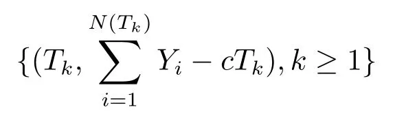
The dual ruin model is de fined as

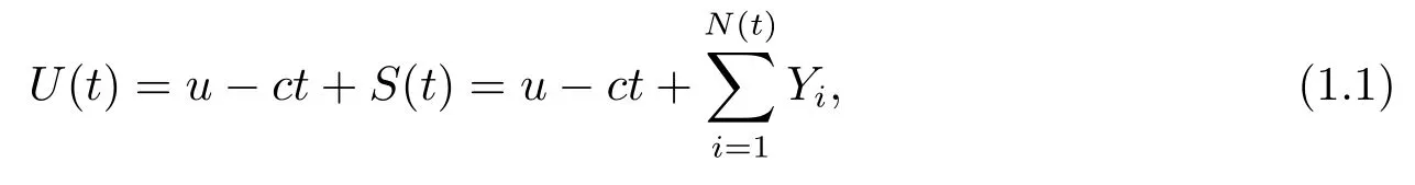
whereu≥0 represents the initial surplus,cis expense rate and the the aggregate revenueS(t)represents the compound Poisson process,given by the Poisson parameterλ.The gain amounts{Yi,i≥1}(independent of{Nt,t≥0})is a sequence of independent and identically distributed(i.i.d)positive random variables with common density functionfY(y).The corresponding Laplace transform of common distributionYis

A hot topic about risk model is the expected discounted dividends until ruin,which is studied thoroughly in many other papers.Avanzi et al.[1]studied the optimal dividends under the barrier strategy;Ng[2]considered discounted dividends in the dual model with a dividend threshold;Albrecher et al.[3]further discussed dividend payments with tax payments.These papers considered the model with exponential inter-event times while some other papers are based on Erlang(n)distributed inter-event times(see Albrecher et al.[4],Yang and Sendova[5]and Eugenio et al.[6]).

In practice,the company’s board checks the surplus regularly and then decides whether to pay dividends to shareholders.Thus dividends may be paid to shareholders only inspecial times.As shown in Avanzi et al.[7],the dual model with Erlang(n)distributed observation times is provided.They assumed that the ruin happens as long as the surplus falls below the zero level.In fact,even if the surplus is negative,the management are no aware of bankruptcy and keep this business alive due to the continuity of business.Thus,only with negative assets in the special times can company go bankrupt(see Albrecher et al.[8]).Peng et al.[9]considered dividend payments in the dual model with exponentially distributed observation times,note that ruin and dividends can only be observed at these random observation times.In this paper,we consider the dual model based on the method of Albrecher et al.[8]who studied the classical risk model with random observation times.

We assume the dual model can only be observed at times{Zk}∞k=1,at which ruin and dividend occur.Constant dividend barrier strategy is implemented.If the surplus exceeds the barrierb＞0 at the timesZk,the excess is paid out immediately as a dividend.Otherwise,there is no dividend payments.

LetTk=Zk−Zk−1(Z0is not assumed to be a dividend decision time),and assume thatis an i.i.d.sequence distributed as a genericr.v.Tand independent of{N(t)}t≥0andThe common distributionTis Erlang(n)distributed with density

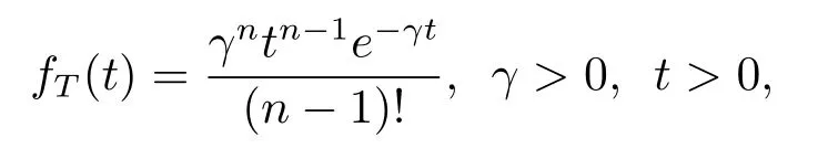
and corresponding Laplace transform has the form

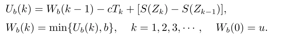
We denote the sequences of surplus levels at the time pointsandbyandrespectively,i.e.,{Ub(k)}and{Wb(k)}are the surplus levels at thek-th observation before(after,respectively)potential dividends are paid.

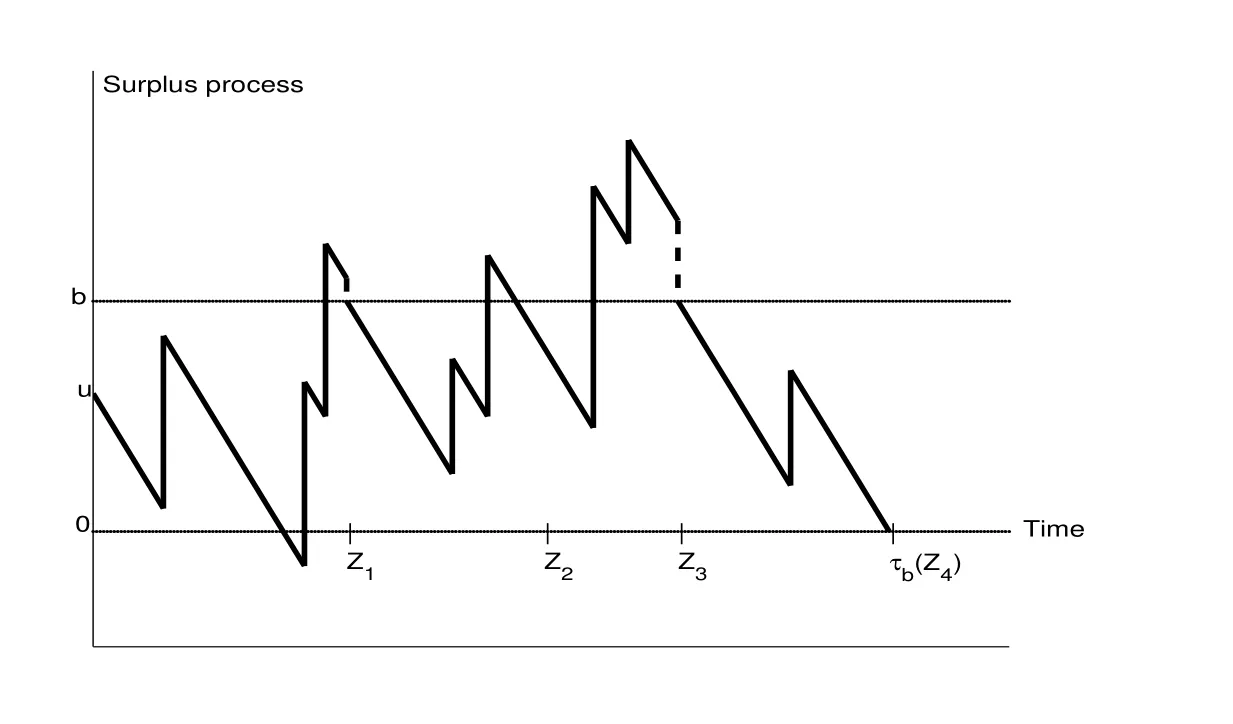
Figure 1:Typical sample path of the dual model under randomized observation

The time of ruin is de fined byτb=Zkb,wherekb=inf{k≥1,Wb(k)≤0}is the number of observation intervals before ruin.Then we have the recursive relation

A sample path under the present model is depicted in Figure 1.

The total discounted dividend payments until ruin for a discount rateδ≥0 are

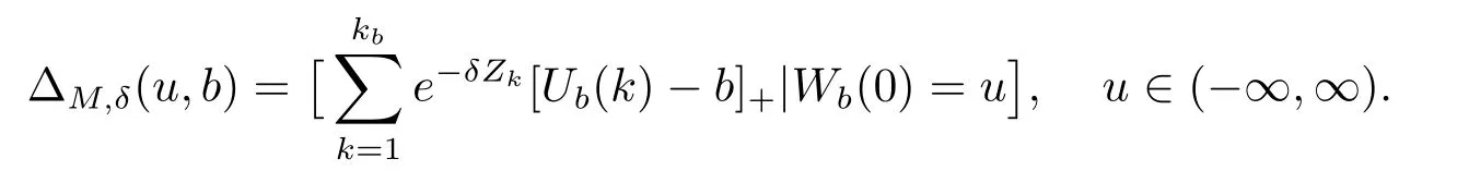
With time 0 an observation time,the total discounted dividend payments until ruin are represented by

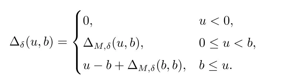
In particular,the distribution of ΔM,δ(u,b)for 0≤u＜balready determines Δδ(u,b)for arbitraryu.

We assume that time 0 is not a dividend decision time.The total expected discounted dividends are

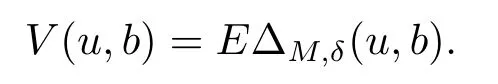
Depending on the value of the initial surplus,de fine

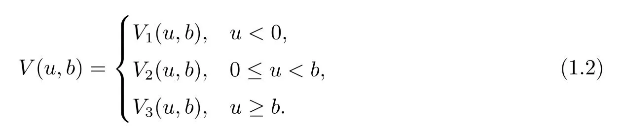
The rest of this paper is organized as follows:in Section 2,we derive and solve the integral equations satisfied by the expected discounted dividends until ruin when the Laplace transform of a general gain distribution follows rational case.In Section 3,we obtain explicit form of the expected discounted dividends when jump sizes and inter-observation times follow an exponential distribution.In Section 4,we generalize the results to the case that the interobservation times are Erlang(2)distributed.In addition,numerical illustrations for the e ff ect of model parameters on the expected value of the discounted dividends are studied and image description is given.

2 Discounted Dividends V(u,b)

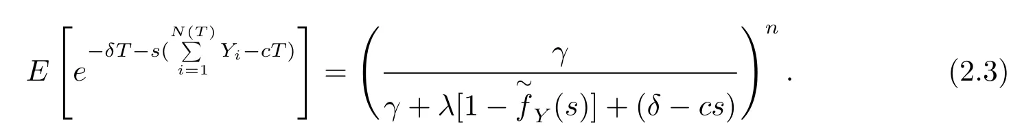
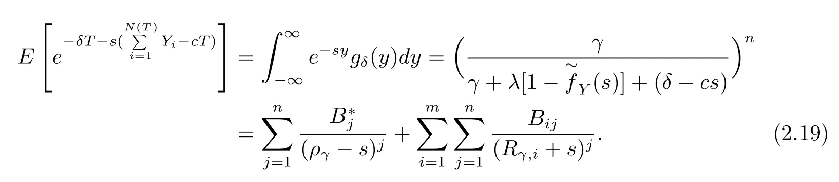
Due to the Markovian structure of{Ut}t≥0,the sequence of pairs

is i.i.d with genetic distributionand joint Laplace transform

As in Albrecher et al.[8],we write

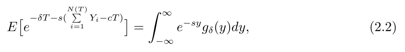
wheregδ(y)(−∞＜y＜∞)represents the discounted density of the incrementbetween successive observation times,discounted at rateδ.According to the assumption that inter-observationThas an Erlang(n)distribution,eq.(2.1)is rewritten as

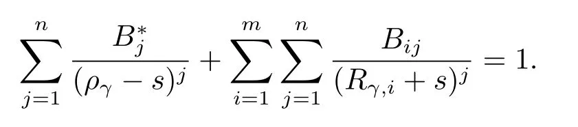
There are zeros in the denominator above,namely,the roots of the equation

in which there is a unique positive rootργ ＞0.To make calculation easier,we use the notation

with continuity conditionV1(0,b)=V2(0,b)andV2(b,b)=V3(b,b).

The quantitiesgδ,−(y)andgδ,+(y)will not always have a tractable form,but iffY(y)has a rational Laplace transform,i.e.,

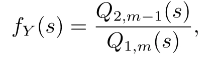
whereQ1,m(s)is a polynomial insof degree exactlymwith leading coefficient of 1 andQ2,m−1(s)is a polynomial insof degree at mostm−1(and the two polynomials have distinct zeros).From Albrecher et al.[10],it follows that

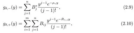
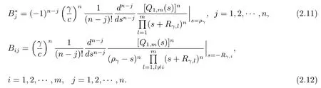
where−Rγ,1,−Rγ,2,···,−Rγ,mare themroots of eq.(2.4)with negative real parts and the constantsB∗jandBijare given by

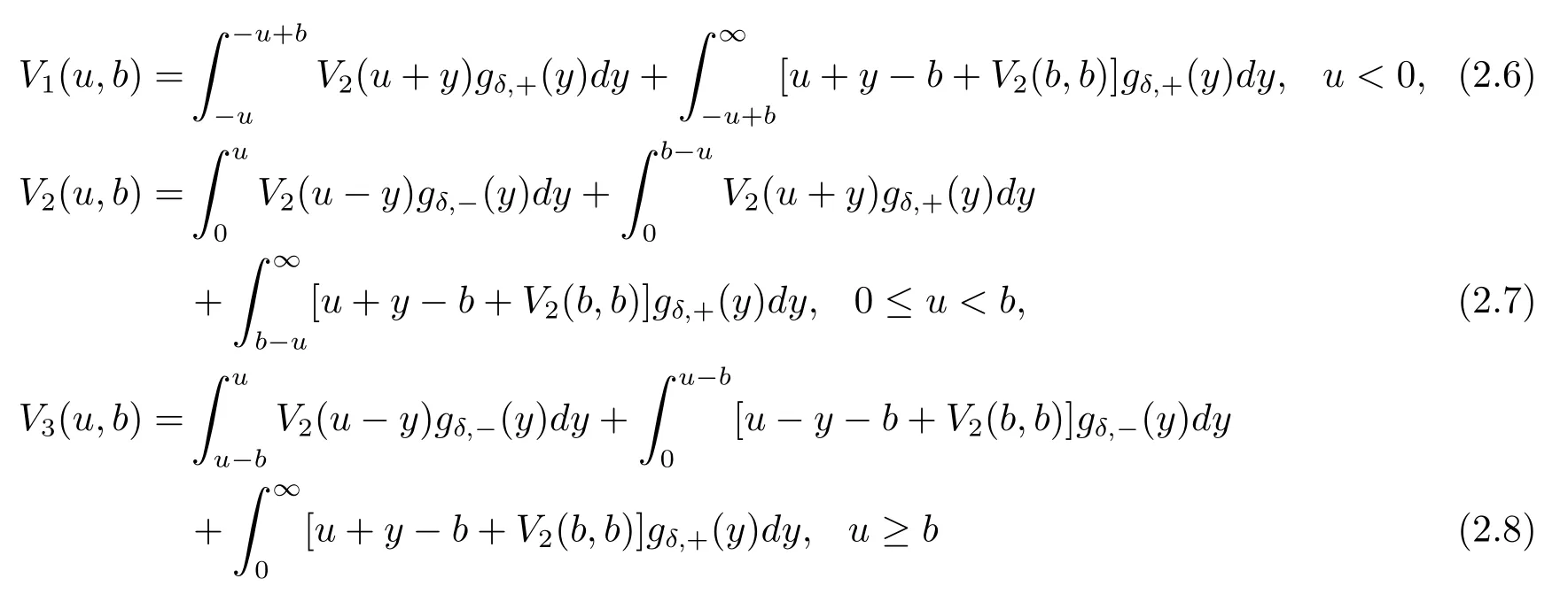
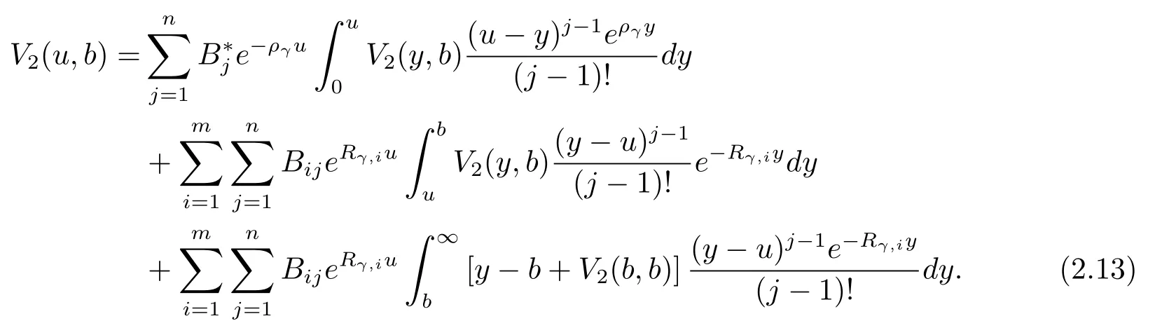
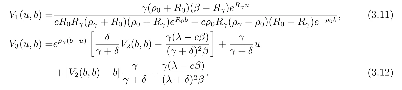
In view of eqs.(2.6)–(2.8),the expression forV1(u,b)andV3(u,b)are closely associated withV2(u,b).So we deriveV1(u,b)andV3(u,b)easily by substituting back the solution forV2(u,b)into eq.(2.6)and eq.(2.8).

Substitution of eq.(2.9)and eq.(2.10)into eq.(2.7)yields,after rearranging terms,

wherekpis the multiplicity of the rootαpand satisfies the equationAs for this case,the method is analogous as follows.Substituting eq.(2.14)into eq.(2.13),the f i rst integral on the right-hand side of eq.(2.13)is evaluated as

Similarly,the second integral in eq.(2.13)is given by

while the third integral in eq.(2.13)is written as

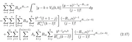
Putting back eqs.(2.15)–(2.17)into eq.(2.13),equating coefficients ofeαpuleads to

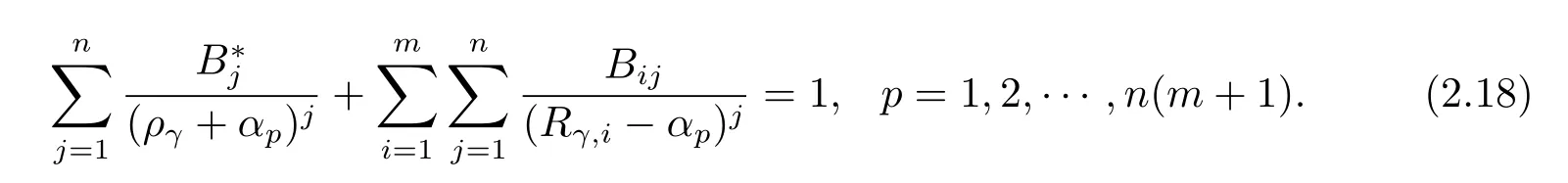
Substitution of eq.(2.9)and eq.(2.10)yields the requirement that

In comparison with eq.(2.18)above,we may conclude thatare the opposite numbers to the roots of the equation

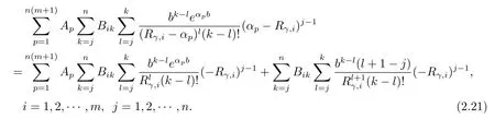
Finally,equating coefficients ofuj−1e−ργuyields

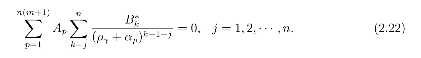
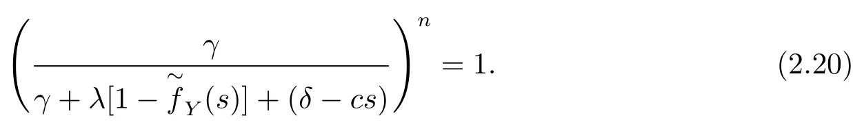
Consequently,we have eq.(2.20)to solve forMoreover,notice that there is a system ofm×n+n=n(m+1)equations for the constantsgiven by eq.(2.21)and eq.(2.22).Hence,the expression forV2(u,b)is obtained easily.

3 The Case That Jump Sizes and Inter-Observation Times are Exponential

In the case thatfY(y)=βe−βy,andfT(t)=γe−γt,eq.(2.4)reduces to

in which there is a positive rootργand a negative root−Rγ(Rγ＞0).Then we may simplify eq.(2.20)to

with a positive rootρ0and a negative root−R0.

From eq.(2.9)and eq.(2.10),it follows that

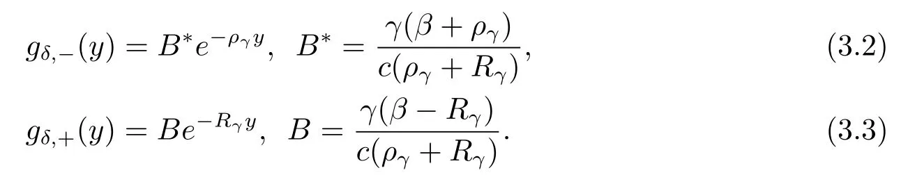
Putting backgδ,−(y)andgδ,+(y)above into the original integral eqs.(2.6)–(2.8)yields

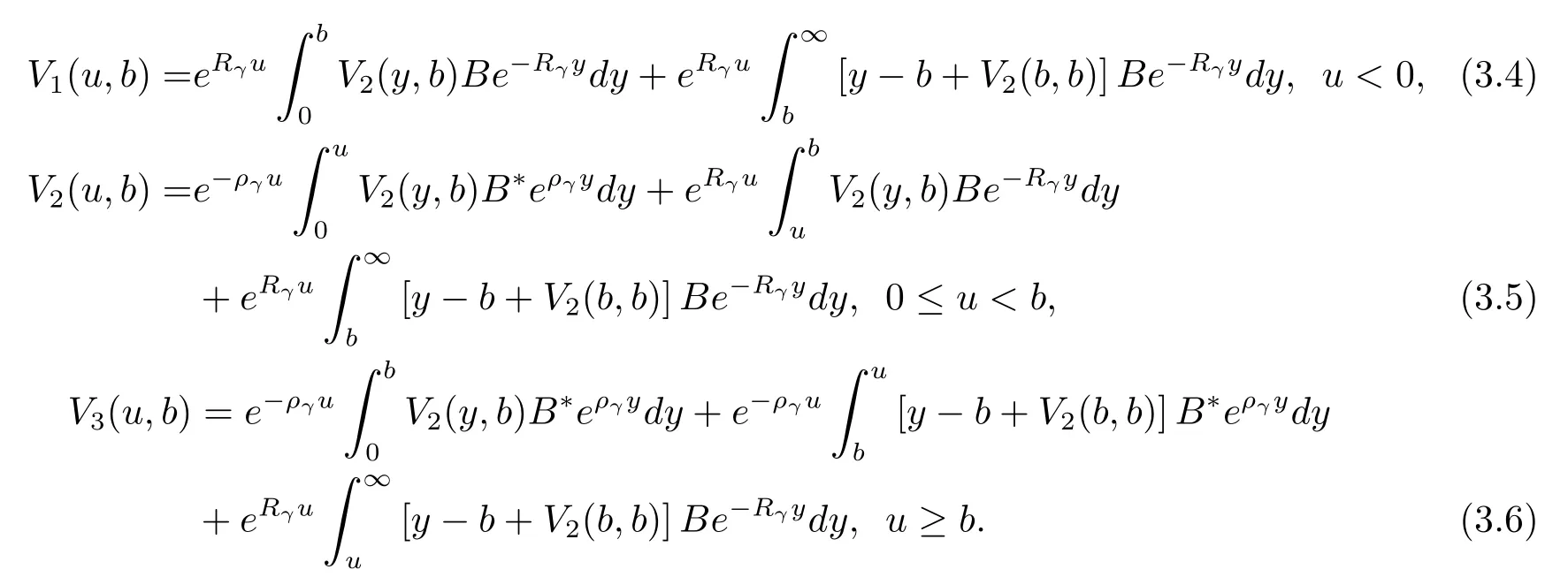
Furthermore,on combining with the conclusion mentioned at the end of Section 2 and the simplified eq.(3.1),the solution forV2(u,b)can be expressed as

SubstitutingV2(u,b)above into eq.(3.5)and comparing the coefficients ofe−ργuandeRγ(u−b)leads to

丁振军表示，尽管近年来市场经历着一些改变，但是欧化农业坚持不变的是产品的品牌、生产线、生产团队、生产控制，特别是产品的品质不会改变。

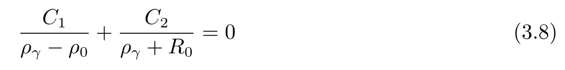
and

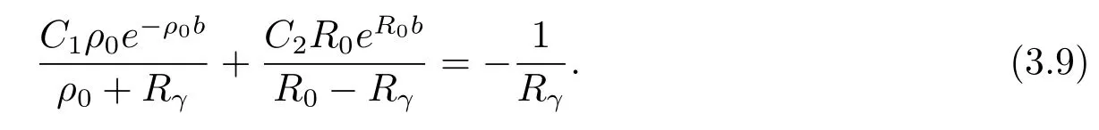
Therefore,we have two linear equations satisfied byC1andC2.After some calculations,we have

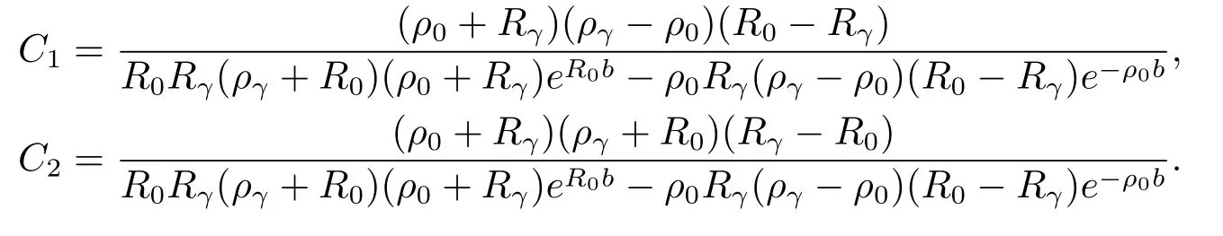
Hence we get

PuttingV2(u,b)above into eqs.(3.4)and(3.6),we obtain

It should be mentioned that using different method we derive the same results as that given by Peng et al.[9].

4 The Case That Jump Sizes are Exponential and Inter-Observation Times are Erlang(2)Distributed

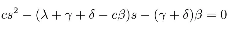
In the case thatfY(y)=βe−βyandfT(t)=γ2te−γt,eq.(2.4)is equivalent to

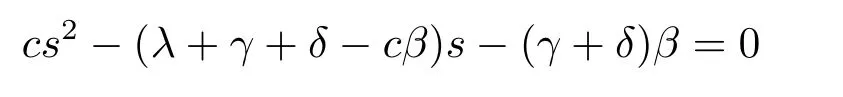
in which there are four rootsρ0,−R0,ρ∗γand−R∗γ.

By eqs.(2.9)and(2.10),we immediately obtain

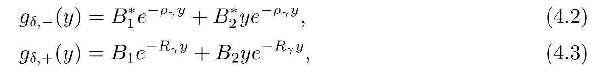
where the constantsB∗1,B∗2,B1,B2are given by

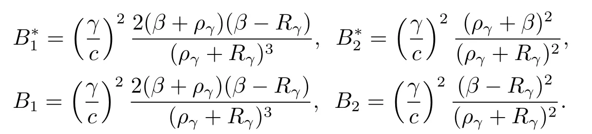
Substituting back eqs.(4.2)and(4.3)into eq.(2.7)produces

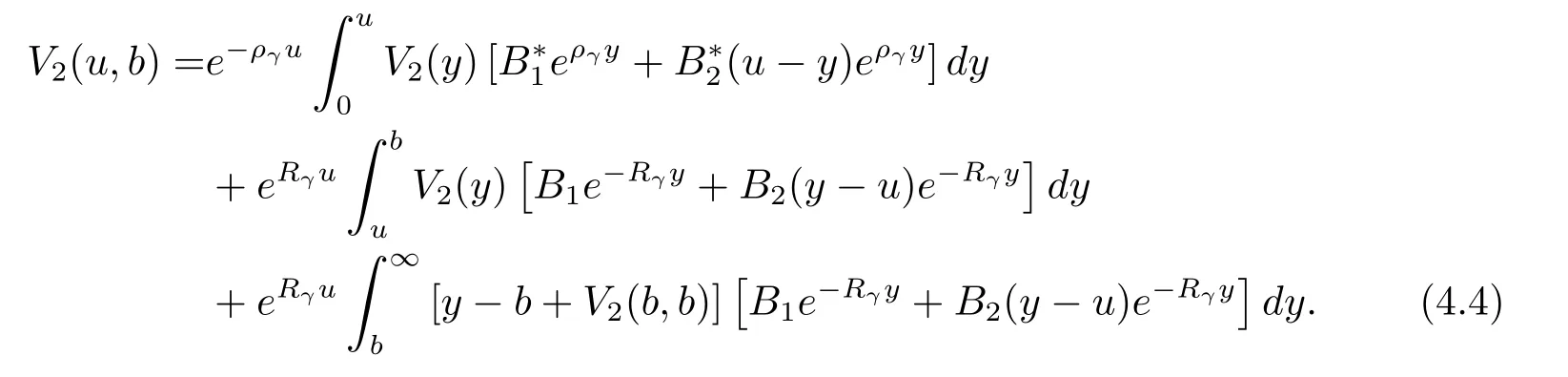
Furthermore,the expression combined with the conclusion discussed before and eq.(4.1)indicates

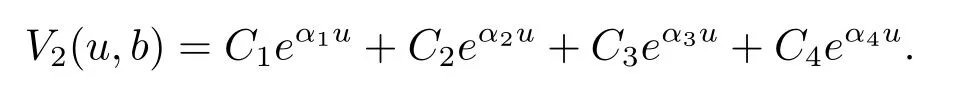
Hence,the solution of eq.(4.4)has the explicit form

PuttingV2(u,b)above into eq.(4.4)and equating coefficients ofue−ργuleads to

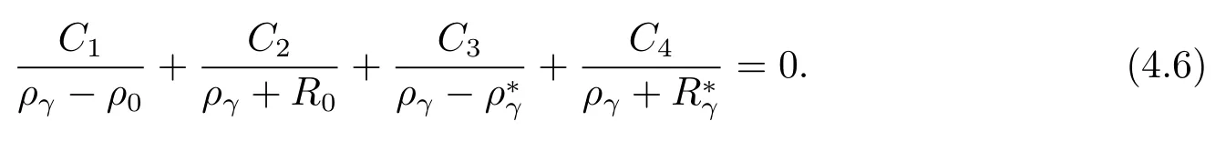
Equating coefficients ofe−ργuleads to

Equating coefficients ofueRγ(u−b)leads to

Equating coefficients ofeRγ(u−b)leads to

Therefore,we have a system of linear eqs.(4.6)–(4.9)for the four remaining constantsC1,C2,C3,C4(only with givenb).

Example 1LetT～Erlang(2,2),λ=1,c=0.8,δ=0.05 andβ=1.The solution of eq.(4.1)are

and we have

Figure 2:V2(u,b)as a function of b for u=0,1,2,3,4,5(from bottom to top)

At the end of this section,we use the following numerical examples to discuss the impact of the model parameters on the expected total dividend payments.Table 1 gives some numerical values ofV2(u,b)and Figure 2 depicts the behavior ofV2(u,b)as a function ofbfor some given values of initial capitalu.The top curve corresponds tou=5,and the next one corresponds tou=4 and so on.Combining both together,we find that dividends increase asuincreases for each fixedb.Observing carefully,V2(u,b)appears to increase withbinitially and decrease afterwards ifuis small.Further,with initial capitalubigger,V2(u,b)is a monotonically decreasing function ofb.

Table 1:Exact values for the expectation V2(u,b)of the discounted dividend payment

[1]Avanzi B,Gerber H U,Shiu E.Optimal dividends in the dual model[J].Insur.Math.Econ.,2007,41(1):111–123.

[2]Andrew C Y Ny.On a dual model with a dividend threshold[J].Insur.Math.Econ.,2009,44(2):315–324.

[3]Albrecher H,Badescu A,Landraiult D.On the dual risk model with tax payments[J].Insur.Math.Econ.,2008,42(3):1086–1094.

[4]Albrecher H,Claramunt M M,Marmol M.On the distribution of dividend payments in a Sparre-Andersen model with generalized Erlang(n)interclaim times[J].Insur.Math.Econ.,2005,37(2):324–334.

[5]Yang C,Sendova K P.The ruin time under the Sparre-Andersen dual model[J].Insur.Math.Econ.,2014,54:28–40.

[6]Eugenio V R,Rui M R C,Alfredo D E.Some advances on the Erlang(n)dual risk model[J].ASTIN Bulletin,2015,45(1):127–150.

[7]Avanzi B,Cheung E C K,Wong B,Woo J K.On a periodic dividend barrier strategy in the dual model with continuous monitoring of solvency[J].Insur.Math.Econ.,2013,52(1):98–113.

[8]Albrecher H,Cheung E C K,Thonhauser S.Randomized observation times for the compound Poisson risk model:dividends[J].ASTIN Bulletin,2011,41(2):645–672.

[9]Peng D,Liu D H,Liu Z M.Dividend problems in the dual risk model with exponentially distributed observation time[J].Stat.Probab.Lett.,2013,83(3):841–849.

[10]Albrecher H,Cheung,E C K,Thonhauser S.Randomized observation periods for the compound Poisson risk model:the discounted penalty function[J].Scand.Actuar.J.,2013,6:424–452.

观察时间服从Erlang(n)分布的对偶模型红利支付

刘 艳1,戚 虎1,戚攀攀2
(1.武汉大学数学与统计学院,湖北武汉 430072)
(2.郑州大学数学与统计学院,河南郑州 450001)

本文研究了观察时间服从Erlang(n)分布的对偶模型红利支付问题.在收益额的拉普拉斯变换是有理拉普拉斯变换的情况下,获得了破产之前总贴现红利V(u;b)的求解方法.该结果推广了文献[8]的相应结论.

对偶模型;观察时间;拉普拉斯变换;贴现红利

O211.6

60E10;62M40;62P05

A

0255-7797(2017)06-1189-12

date:2015-07-25Accepted date:2015-11-18

Biography:Liu Yan(1977–),female,born at Tai’an,Shandong,associate professor,major in probability theory and financial insurance.