Jakob Maljaars, Robert Jan Labeur, Matthias Möller, Wim Uijttewaal

1. Environmental Fluid Mechanics Section, Faculty of Civil Engineering and Geosciences, Delft University of Technology, Delft, The Netherlands, E-mail: j.m.maljaars@tudelft.nl

2. Department of Applied Mathematics, Delft University of Technology, Delft, The Netherlands

Development of a hybrid particle-mesh method for simulating free-surface flows*

Jakob Maljaars1, Robert Jan Labeur1, Matthias Möller2, Wim Uijttewaal1

1. Environmental Fluid Mechanics Section, Faculty of Civil Engineering and Geosciences, Delft University of Technology, Delft, The Netherlands, E-mail: j.m.maljaars@tudelft.nl

2. Department of Applied Mathematics, Delft University of Technology, Delft, The Netherlands

2017,29(3):413-422

In this work the feasibility of a numerical wave tank using a hybrid particle-mesh method is investigated. Based on the fluid implicit particle method (FLIP) a formulation for the hybrid method is presented for incompressible multiphase flows involving large density jumps and wave generating boundaries. The performance of the method is assessed for a standing wave and for the generation and propagation of a solitary wave over a flat and a sloping bed. A comparison is made with results obtained with a well-established SPH package. The tests demonstrate that the method is a promising and attractive tool for simulating the nearshore propagation of waves.

Lagrangian-Eulerian, particle-mesh, free-surface flows, numerical wave flume, incompressible Navier-Stokes

Introduction

The numerical modeling of flow problems in environmental fluid mechanics has made huge progress over the past decades. While Eulerian mesh-based methods are widely used for solving the governing Navier-Stokes equations, Lagrangian particle-based methods such as the smoothed particle hydrodynamics (SPH) method are becoming increasingly popular for problems involving violent free-surface motion[1,2]. Where interface tracking in Eulerian methods requires additional effort, interfaces are naturally captured by Lagrangian particle-based methods. However, the fine particle resolution which is required to obtain good accuracy, and the construction of neighbor particle lists render the Lagrangian particle-based methods computationally much more demanding than Eulerian meshbased methods. On top of that, enforcing the incompressibility constraint in particle-based methods is not trivial[3,4]. Therefore, fluids are often assumed to be weakly compressible in particle-based methods which, in combination with explicit time stepping schemes, leads to restrictively small time steps when applied to(nearly) incompressible fluids.

In the late 1950s, Harlow and coworkers introduced the particle-in-cell (PIC) method[5], which combines the advantages of the Eulerian and the Lagrangian approaches. Originally being developed for hydrodynamic problems involving large distortions or compressions, particle-mesh methods have seen a wide variety of applications ever since, including the simulation of free-surface flow problems[6,7]. Various fundamental improvements to the original PIC method have been proposed over the past decades. The Fluid Implicit Particle (FLIP) method was introduced by Brackbill in order to alleviate the numerical diffusion present in the original PIC method[8], and Sulsky introduced another variant of PIC, termed material point method (MPM), to simulate history dependent material behavior[9].

This work outlines a hybrid Lagrangian-Eulerian (particle-mesh) method for simulating incompressible fluid flows by presenting a generic formulation for the particle-mesh interaction and a strategy for efficiently solving the (Navier-Stokes) equations on the background mesh. Building upon FLIP[8]and PIC[5]concepts, the proposed method has the combined advantages of Eulerian mesh-based and Lagrangian particlebased methods. For the proposed particle-mesh interaction procedure, the method is more geared towards amesh-based method than, e.g., the MPM and SPH.

More specifically, this work aims at developing a hybrid particle-mesh numerical wave model, where both the air- and the water-phase are discretized by means of Lagrangian particles. Several issues to achieve this objective are addressed in this work: particularly, the implementation of wave-making boundary conditions and a method to deal with sharp discontinuities in material properties are presented. The practical feasibility of the approach is assessed by presenting two different numerical tests, in which a comparison is made between analytical results and/or results obtained with the DualSPHysics package[10].

1. Governing equations

The motion of an incompressible fluid in a domain Ω⊂Rd, in which 1≤ d≤3is the spatial dimension, and time intervalI =(t0,tN)is described by the incompressible Navier-Stokes equations, comprising both the momentum balance and the incompressibility constraint. For Newtonian fluids, these equations read:

in whichudenotes the flow velocity,ρthe density, p the pressure,fthe body force and the viscous stress tensor is given byσ=2µ ∇suwith the symmetric gradient operator ∇s(⋅)= 1/2 ∇(⋅)+ 1/2 ∇(⋅)Tand µthe dynamic viscosity.

In the framework of the hybrid particle-mesh me- thods, Eqs.(1), (2) represent the equations to be solved on the background mesh.

2. Model formulation

A hybrid particle-mesh method typically consists of the following steps:

(1) Particle-mesh projection, data from the scattered particles is projected onto the background mesh in order to reconstruct continuous density and velocity fields.

(2) Solving the equations at the mesh, the continuum equations (Eqs.(1), (2)), are solved at the Eulerian background mesh.

(3) Mesh-particle projection, given the solution obtained in Step 2, particle properties are updated. For immiscible, incompressible fluids this yields an update of the particle velocity (being representative for the change in particle momentum).

(4) Particle advection, the particle position is updated by moving the particles with an advective velocity.

Step 2 and 4 are entirely performed at the mesh and particle level, respectively. Step 1 and 3 take care of the coupling between particles and the background mesh. A formulation for the 4 different steps involved is presented below.

2.1 Particle projection to the mesh

For the transfer of particle properties onto the background mesh, a least-squares fitting approach is adopted following[11,12], which yields a smooth representation of properties on the mesh. Similar techniques have been developed in the MPM community[13,14], to overcome the noisy behavior of classical MPM[9]where mass integrals are replaced by summations over the discrete set of particles. An extensive discussion of the least-squares approach can be found in Refs.[11] and [15]. In essence, the continuous density and velocity fieldsρanduare approximated in finitedimensional scalar- and vector-valued function spacesVh⊂L2(Ω )andVh⊂L2(Ω ), that is

where Ni(x)are the piecewise polynomial basis functions for the density field and the velocity field defined on the cells of the background mesh. Moreover, ρianduidenote the nodal degrees of freedom and the summation runs over the number of nodal density unknownsnρand velocity unknowns nu, respectively.

Given the particle density ρpand particle velocityup, the corresponding fields on the background mesh are obtained by solving the least-squares projection

for ρjandujthe nodal density and velocity unknowns at the background mesh, respectively. In theseequations,Ni,jare nodal basis functions which, in Eqs.(5) and (6) are evaluated at the particle positionxp, furthermore, the summation runs over the set of particles inΩ.

Since the finite-dimensional function spaces for the density and the velocity are only required to be square integrable, the reconstructed fieldρh(x)and fielduh(x)can be discontinuous across cell boundaries.

2.2 Solving the equations at the mesh

Since the Lagrangian particles are used to discretize the advection operator, the governing equations at the Eulerian background mesh (Eqs.(1), (2) reduce to the unsteady Stokes equations. These equations are solved using the fractional-step method suggested in Ref.[16]. In this approach, the equations for the velocity and the pressure are solved sequentially and coupled using an intermediate velocity field. The resulting set of equations is discretized in space using the finite element method, where the density and the velocity are approximated using Eqs.(3), (4) and the pressure pis approximated in the finite-dimensional function spaceQh⊂H1(Ω ), i.e.

with Ni(x)the piecewise polynomial basis functions andpithe nodal degrees of freedom for the pressure. Furthermore, the summation runs over the number of pressure unknownsnp.

The finite element discretization results in the following set of variational equations to be solved at the background mesh (an extensive derivation of below presented fractional-step approach can be found in Ref.[15]): given, find the intermediate velocitysuch that

In these equations, the time level is denoted by the superscriptn with time interval ∆t. The boundary term involvinghis more extensively discussed in Section 2.5. It is important to note that both the velocity, and the densityare obtained from the particle-mesh projection step (Section 2.1), and hence, no information is stored at the mesh between consecutive time steps.

Given the saddle-point nature of the incompressible Navier-Stokes equations, the velocity spaceVhand pressure spaceQhmust satisfy the inf-sup condition[17]in order to avoid spurious pressure modes. In this study, the stableP0P1-element is used, having piecewise-constant velocities and piecewise-linear pressure approximations. Although the proposed method is not restricted to using this particular element, it has the additional advantage in that the particle-mesh mapping becomes a local operation since the piecewise-constant basis functions are used for this projection. As a result, Eqs.(5), (6) result in small, local problems, which can be solved independently for each cell.

For the chosen P0P1-element, one additional complication arises when discretizing the term involving the viscous stress. Using the piecewiseconstant approximation(P0)for the velocity, the symmetric gradient of the velocity field and hence the viscous stress trivially evaluates to zero. In order to overcome this, the viscous stress is projected to a continuous tensor field. Hence, the viscous stress can be obtained as: withsuch thatin which Eq.(12) follows from integration by parts of the right hand side of Eq.(11). Furthermore,uDis the bo undary co ndition prescribed onuhwhere it is noted that settinguD=0leads to a no-slip boundary condition.

The FEniCS finite element package[18]is used for efficiently solving Eqs.(8)-(10) (supplemented with Eq.(12) when viscosity is included).

2.3 Mesh-particle mapping

Solving the set of discrete equations yields a velocity field on the background mesh at the new time step, which can be used to update the velocity carried by the particles. In order to do so, first of all a more detailed piecewise-linear velocity fieldis reconstructed from the piecewise-constant velocity fieldby performing an additional projection step at the background mesh[20]. This results in a velocity fieldwise-linear polynomials associated with the three sublements, having the barycenter of the element as shared node andare the corresponding nodal velocities, Fig.1. Based on the recovered velocity fieldthe particle velocities are updated by adding the mesh velocity increment, which is a common approach in the FLIP method. It is however known that a pure FLIP velocity update can develop noisy particle velocity fluctuations[19]. The fundamental reason underlying this artifact is the larger amount of particle degrees of freedom compared to the number of mesh dofs, hence, the mesh-particle update is essentially an underdetermined problem. These high-frequency fluctuations are absent in the PIC method, in which particle velocities are overwritten by the mesh velocity in every time step. However, this method is known to be diffusive. In order to suppress the high-frequency fluctuations while avoiding the numerical diffusivity, a blended PIC/FLIP update following[19]is used.

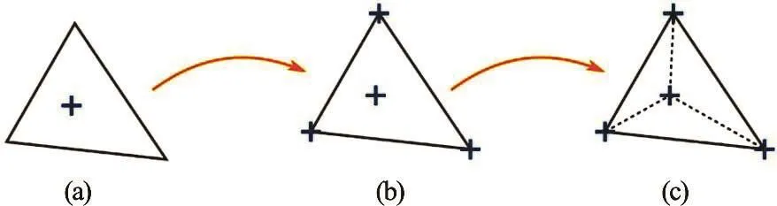
Fig.1 (Color online) Mapping procedure: (a) cell-centered velocity field. (b) velocity mapped to vertices. (c) division into sub-elements around barycenter

Thus, the particle velocity is updated as follows

with the subscript p denoting the particle index andthe mesh velocity increment, whereFurthermore, the PIC fraction is den oted with0 ≤ α≤1.

2.4 Particle advection

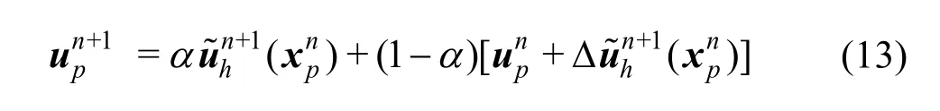
At the end of every time step, the particles are advected by solving the ordinary differential equation for each particle

using the same velocity interpolantas in Section 2.3.

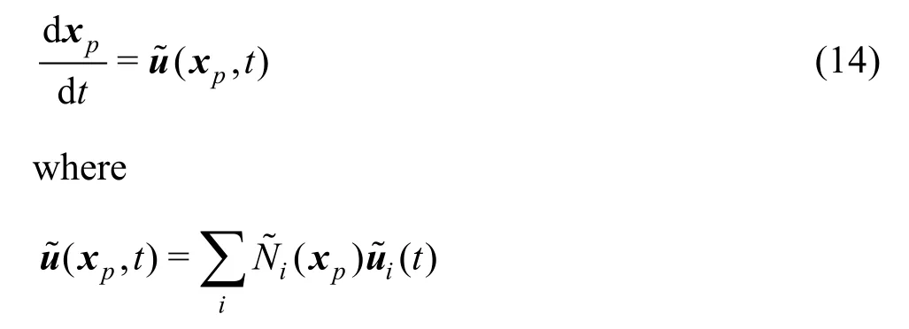
Fig.2 (Color online) Particle trajectories for Point A and B in a solid body rotation

Since this step is responsible for the advection of material properties through the domain, the advection scheme has to be sufficiently accurate. This can be illustrated by a simple example, where particles are passively advected by the velocity fieldwhich describes particle motion on concentric circles around (x0,y0). In Fig.2, the results are presented following the trajectories of two particles, denoted by A and B, usingω= πrad/sand (x0,y0)=(0.5,0.5) after 5 full rotations (i.e., 10 s) for two different time integration schemes. The Courant number for Point B in this numerical experiment is approximately equal to 0.2.

Clearly, the Euler scheme is inaccurate, as particles drift away from the center of rotation. In contrast, the third-order Runge-Kutta (RK3) integration proposed by Ralston[21]succeeds in preserving concentric circle trajectories, therefore, this scheme will be used in the sequel.

2.5 Boundary conditions

2.5.1 Wave-making boundary

Wave making boundaries are of special interest in the context of a numerical wave flume. Recalling the weak form of the Pressure-Poisson equation (Eq.(9)) it is clear that the boundary termnqdΓcan be used to enforce the normal velocity, whereΓNis the part of the domain on which a Neumann condition for the pressure is specified and the boundary velocityhcan be specified according to a wavemaker theory. In order to avoid empty elements (i.e., elements not containing any particles) near the boundary, a moving-mesh approach is used. Since no information is stored at the background mesh between consecutive time steps, moving the mesh does not alter the governing equations. At the top boundary of the numerical flume, the pressure is set to zero in order to simulate an open boundary. Correspondingly, (air)-particles are free to move out- and inward through this boundary during the computation.

2.5.2 Interface condition

The Lagrangian particles naturally track the airwater interface and no additional interface conditions are to be specified. However, in two-phase flow problems, discontinuities in the pressure gradient occur due to the density jump at the interface. Ambiguous definition of the density in elements crossed by the interface, may result in spurious oscillations[22]. To suppress these spurious velocities it is noted that in gravitational equilibrium the pressure gradient term exactly balances the gravitational acceleration, i.e., ρ−1∇ p=g. So although the pressure gradient and the density itself are discontinuous at the interface, the termρ−1∇pis continuous in gravitational equilibrium. Inspired by this observation, the pressure gradient term in Eq.(10) is projected to a piecewise-linear field. In other words, the task is to findr∈Shsuch that

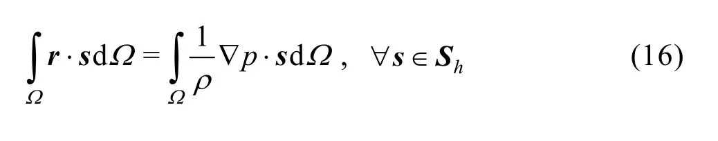
in which the function space

Consequently, the problem for calculating the end-of-step velocity (Eq.(10)) becomes: findsuch that

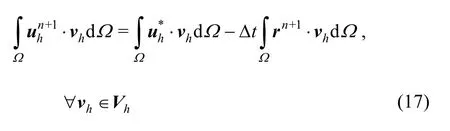
This approach indeed effectively suppresses the spurious velocities near the interface.

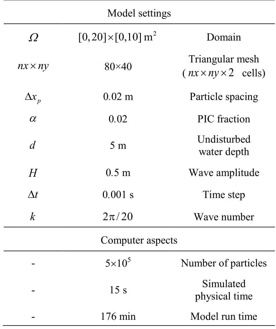
Table 1 Model settings standing wave

3. Numerical examples

3.1 Standing wave

As a first numerical test, a standing wave in a closed basin is considered, which includes the airwater interface. This test provides useful insight in the amount of numerical diffusion and will indicate whether or not the scheme is able to deal with large density differences between the phases. Model results are compared with the analytical expression for the freesurface elevation obtained from linear wave theory.Model settings are listed in Table 1. In addition, the vertical coordinate is denoted withz , with z=0at the still water surface elevation andzassumed to be positive upwards. A small amount of damping is added by blending the FLIP update with a small PIC fraction (see Section 3.3). No detailed investigation of the critical time step was made, therefore a conservative value of∆t=0.001swas used (corresponding to a Courant number of approximately 0.02). It is however noted that this time step size is still typically O(102) larger than in weakly compressible approximations[23].

The simulated air-water interface and the resulting pressure fields for the water-phase are depicted in Fig.3 at two different time instances. The resulting pressure fields are perfectly smooth and no pathological locking effects are observed. Furthermore, the airwater interface is relatively well-maintained, although small disturbances at the free-surface are observed near the inflection points of the cosine wave.

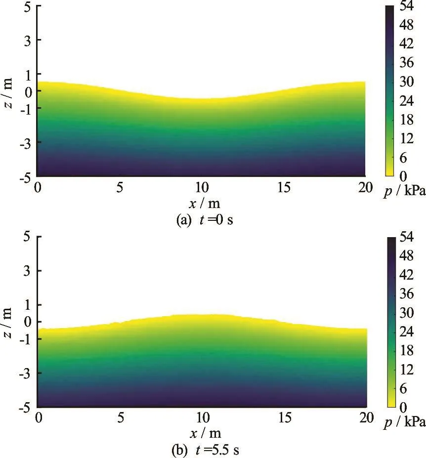
Fig.3 (Color online) Interface positions and pressures in the water phase of a standing wave with H/d=0.1

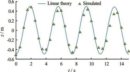
Fig.4 (Color online) Theoretical and simulated amplitudes at x=0.5L

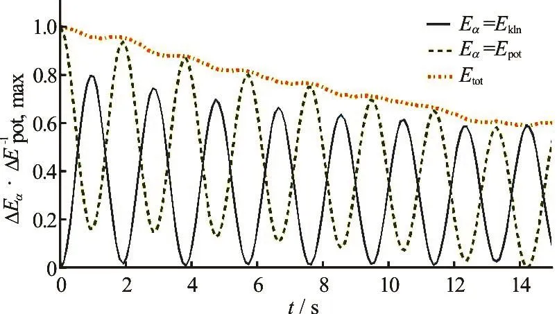
Fig.5 (Color online) Total, kinetic and potential energy in standing wave

The simulated amplitudes are compared at x= 0.5L=10min Fig.4 with the analytical amplitudes following from linear wave theory. A good correspondence between simulated results and analytical values is found, although a slight amplitude decay is observed. The damping present in the scheme is also observed when plotting the potential and the kinetic energy (non-dimensionalized by the potential energy budget), Fig.5. A decay in total particle energy of approximately 40% in four wave periods is observed. This is however smaller than the reported 69% in four wave periods for the SPH implementation presented in Ref.[24], for a comparable problem.

Finally, the simulated pressures are compared to the analytical pressures. To this end, the wave-induced pressure is considered. For linear waves, the total pressure is given by[25]

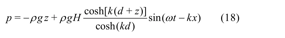
where ρis the density of water,gthe gravitational acceleration andωdenotes the radian frequency which follows from the dispersion relationship. For an explanation of the other symbols, reference is made to Table 1. The first term at the right hand side of Eq.(18) represents the hydrostatic balance, whereas the second term represents the wave-induced pressure, i.e.

Simulated wave-induced pressures are computed by subtracting the hydrostatic component ρgzfrom the total pressure (withz=0at the still water surface elevationd). The resulting values are plotted against the analytical values following from the linear wave theory (Eq.(19)) at x=0.5L=10mafter a half wave period (t ≈1.7s)and a full wave period (t ≈3.8s). Results are depicted in Fig.6, showing avery good correspondence both at a time instance of maximum elevation (t ≈1.7s)and minimum elevation(t ≈3.8s). The slight underestimation of the wave-induced pressure of approximately 500 Pa for the maximum elevation should be put into perspective by noting that this difference is only around 1% of the maximum pressure (see Fig.3).

Fig.6 (Color online) Wave-induced pressure in standing wave below

3.2 Propagation of a solitary wave

As a test case to assess the performance of the scheme for large amplitude problems, the generation and propagation of a solitary wave over a flat (Section 3.2.1) and over a sloping bed (Section 3.2.2) is considered. For the propagation over the flat bed, a comparison is made with approximate analytical expressions[23]and results obtained using the open source DualSPHysics package[10].

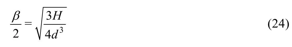
The forced generation of a solitary wave by means of piston wave makers can be found in Refs.[26] and [27]. Based on these references, the boundary displacement xb(t)and boundary velocity are respectively given by In these equations,τis a characteristic time duration for the paddle motion, andSthe paddle stroke, respectively given by:with the wave celerity given by c = g(d + H)and H anddare the wave height and the undisturbed water depth, respectively. Furthermore,βis the socalled outskirts decay coefficient, defined as

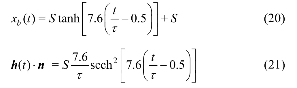
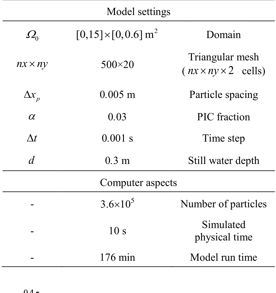
Table 2 Model properties solitary wave generation

Fig.7 (Color online) Comparison between the analytical, the hybrid particle-mesh and the DualSPHysics solution for the generated solitary wave at t=8s

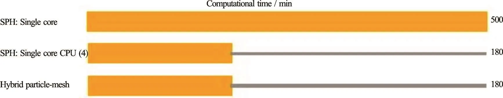
Fig.8 (Color online) Approximate computational times for the DualSPHysics model in various computing configurations and the developed hybrid particle-mesh method

Given the boundary motion, the surface elevation ζis approximated by

3.2.1 Solitary wave propagation over a flat bed

For the test case involving a flat bed, a solitary wave is generated in the domain initially defined byΩ=[0,15]×[0,0.6]m2. A time step ∆t=0.001sis used, corresponding to a Courant number of approximately 0.02. Other model parameters and computational aspects are listed in Table 2. The model is run for two different dimensionless amplitudes H/d =0.2and H/d=0.35.

Results for both runs are depicted in Fig.7 at t=8 s. A good agreement is observed between simulated and analytical results, although model results are slightly lagging behind the analytical solution, which can be attributed to numerical diffusion. However, this numerical diffusion is much more pronounced for the SPH runs obtained with DualSPHysics and using a comparable model setup, Fig.7. In order to mimic the inviscid case in DualSPHysics, the artificial viscosity (representing the viscosity term and enhancing numeri- cal stability) is set to 0. Clearly, results obtained with the DualSPHysics package (using the same particle spacing) are much more diffusive than results obtained with our hybrid particle-mesh method.

In terms of computational effort, the developed model is able to compete with the DualSPHysics implementation, as shown in Fig.8: running the hybrid particle-mesh simulation on a single core results in a computational time of approximately 180 min, compared to approximately 500 min for the DualSPHysics computation on a single core. The gain in CPU time can be partly attributed to the less restrictive time step requirements in the incompressible hybrid particlemesh method compared to the weakly-compressible SPH model. Based on the presented comparison, it can be concluded that the results obtained with the hybrid particle-mesh method are encouraging both in terms of accuracy and computational efficiency.

3.2.2 Solitary wave propagation over a sloping bed

A final example showing the capabilities of the model, is the breaking of a solitary wave on a submerged bar, placed in a domain with a horizontal and vertical base of 13 m×1 m. An unstructured, boundaryfitted triangular mesh is used for this simulation, containing approximately 25 000 cells. Around 25 particles are initially placed in each cell. In the domain, a solitary wave is generated with a relative amplitude H/d=0.625. A time step of 0.001 s is used. Other model properties including the computational aspects are listed in Table 3.

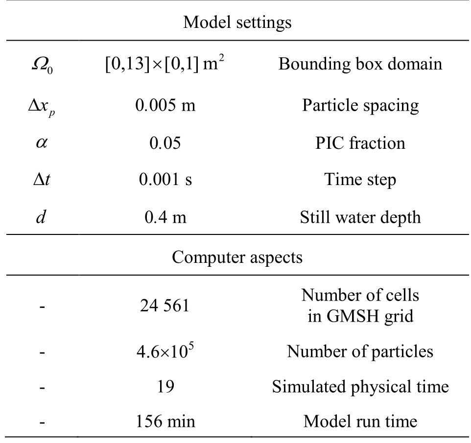
Table 3 Model properties breaking wave simulation

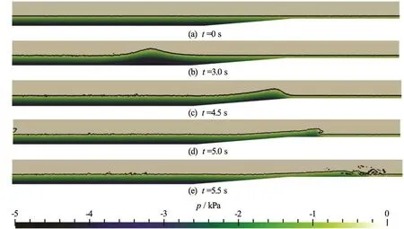
Fig.9 (Color online) Soliton propagation including breaking on a submerged bar. Color shading indicates the pressures at the background mesh

The process of wave propagation and wave breaking is presented in Fig.9, qualitatively revealing the important nearshore wave processes: wave steepening (shoaling) around t =4.5s, wave plunging around t =5s, and wave breaking around t=5.5s. Although not validated quantitatively here, the test reveals the capability of hybrid particle-mesh methods to simulate the wave propagation processes, including wave breaking.

4. Conclusions

In this study, a hybrid particle-mesh approach for incompressible fluid flows was formulated and tested for various free-surface benchmark tests. The method was shown to combine various advantages of an Eulerian mesh-based approach (enforcing incompressibility, fast and efficient solvers) with the advantages of a pure Lagrangian particle-based approach (tracking interfaces of complex topography).

Due to the implicit treatment of the pressure, smooth and accurate pressure fields are obtained as shown for the standing wave test case. Additional advantage of this approach compared to the weakly compressible approach is the mild time step requirement, thus rendering the method an attractive alternative to pure particle-based methods such as SPH when setting up a numerical wave tank.

It is realized that this work presents only a first investigation of the feasibility for efficiently using particle-mesh methods in simulating free-surface flows in the context of a numerical wave flume. Various fundamental aspects need therefore to be addressed in future work, including first and foremost the physical and theoretical underpinnings of the method. Future work will also focus on various numerical aspects (e.g., convergence issues and the minimal number of particles required in a cell for which results are still accurate) and a further quantitative assessment of model results.

Acknowledgements

The NWO (Netherlands Organisation for Scientific Research) is acknowledged for their support through the JMBC-EM Graduate Programme research grant.

[1] Monaghan J. Simulating free surface flows with SPH [J]. Journal of Computational Physics, 1994, 110(2): 399-406.

[2] Colagrossi A., Landrini M. Numerical simulation of interfacial flows by smoothed particle hydrodynamics [J]. Journal of Computational Physics, 2003, 191(2): 448-475.

[3] Chen Z., Zong Z., Liu M. B. et al. A comparative study of truly incompressible and weakly compressible SPH methods for free surface incompressible flows [J]. International Journal for Numerical Methods in Fluids, 2013, 73(9): 813-829.

[4] Marrone S., Colagrossi A., Antuono M. et al. An accurate SPH modeling of viscous flows around bodies at low and moderate Reynolds numbers [J]. Journal of Computational Physics, 2013, 245(1): 456-475.

[5] Evans M., Harlow F., Bromberg E. The particle-in-cell method for hydrodynamic calculations [R]. Technology Report, Los Alamos, USA: Los Alamos Scientific Laboratory, 1957.

[6] Kelly D. M., Chen Q., Zang J. PICIN: A particle-in-cell solver for incompressible free surface flows with two-way fluid-solid coupling [J]. Journal on Scientific Computing, 2015, 37(3): 403-424.

[7] Zhang F., Zhang X., Sze K. Y. et al. Incompressible material point method for free surface flow [J]. Journal ofComputational Physics, 2017, 330: 92-110.

[8] Brackbill J., Ruppel H. FLIP: A method for adaptively zoned, particle-in-cell calculations of fluid flows in two dimensions[J]. Journal of Computational Physics, 1986, 65(2): 314-343.

[9] Sulsky D., Chen Z., Schreyer H. A particle method for history-dependent materials [J]. Computer Methods in Applied Mechanics and Engineering, 1994, 118(1-2): 179- 196.

[10] Crespo A., Dominguez J., Rogers B. et al. DualSPHysics: Open-source parallel CFD solver based on smoothed parti- cle hydrodynamics (SPH) [J]. Computer Physics Commu- nications, 2015, 187: 204-216.

[11] Subramaniam S., Haworth D. C. A probability density function method for turbulent mixing and combustion on three dimensional unstructured deforming meshes [J]. International Journal of Engineering Research, 2000, 1(2): 171-190.

[12] Edwards E., Bridson R. Detailed water with coarse grids [J]. ACM Transactions on Graphics, 2014, 33(4): 1-9.

[13] Steffen M., Kirby R. M., Berzins M. Analysis and reduction of quadrature errors in the material point method (MPM) [J]. International Journal for Numerical Methods in Engineering, 2008, 76(6): 922-948.

[14] Tielen R. High order material point method [D]. Master Thesis, Delft, The Netherlands: Delft University of Technology, 2016.

[15] Maljaars J. A hybrid particle-mesh method for simulating free surface flows [D]. Master Thesis, Delft, The Netherlands: Delft University of Technology, 2016.

[16] Chorin A. J. Numerical solution of the Navier-Stokes equations [J]. Mathematics of Computation, 1968, 22(104): 745-762.

[17] Brezzi F., Fortin M. Mixed and hybrid finite element methods [M]. Berlin, Germany: Springer-Verlag, 1991.

[18] Logg A., Mardal K.-A., Wells G. N. Automated solution of differential equations by the finite element method [M]. Berlin, Germany: Springer-Verlag, 2012.

[19] Bridson R. Fluid simulation for computer graphics [M]. Boca Raton, USA: CRC Press, 2008.

[20] Ando R., Thürey N., Wojtan C. Highly adaptive liquid simulations on tetrahedral meshes [J]. ACM Transactions on Graphics, 2013, 32(4): 1-10.

[21] Ralston A. Runge-Kutta methods with minimum error bounds [J]. Mathematics of Computation, 1962, 16(80): 431-437.

[22] Wemmenhove R. Numerical simulation of two-phase flow in offshore environments [D]. Doctoral Thesis, Groningen, The Netherlands: University of Groningen, 2008.

[23] Wieckowski Z. Enhancement of the material point method for fluid-structure interaction and erosion [R]. Research Project Report, Delft, The Netherlands: Deltares, 2013.

[24] de Wit L. Smoothed particle hydrodynamics. A study of the possibilities of SPH in hydraulic engineering [D]. Master Thesis, Delft, The Netherlands: Delft University of Technology, 2006.

[25] Holthuijsen L. H. Waves in oceanic and coastal waters [M]. Cambridge, UK: Cambridge University Press, 2010.

[26] Goring D. G. Tsunamis: The propagation of long waves onto a shelf [D]. Doctoral Thesis, Pasadena, USA: California Institute of Technology, 1978.

[27] Katell G., Eric B. Accuracy of solitary wave generation by a piston wave maker [J]. Journal of Hydraulic Research, 2002, 40(3): 321-331.

10.1016/S1001-6058(16)60751-5

February 14, 2017, Revised March 20, 2017)

*Biography:Jakob Maljaars, Male, Ph. D. Candidate