Zhuang-ming Zhao (赵庄明), Ping Huang (黄平), Shao-tian Li (李少钿)

1.South China Institute of Environmental Sciences, the Ministry of Environmental Protection of PRC, Guangzhou 510655, China, E-mail: zhaozhuangming@scies.org

2.Department of Environmental Science, School of Environmental Science and Engineering, Sun Yat-sen University, Guangzhou 510275, China

Lattice Boltzmann model for shallow water in curvilinear coordinate grid＊

Zhuang-ming Zhao (赵庄明)1, Ping Huang (黄平)2, Shao-tian Li (李少钿)2

1.South China Institute of Environmental Sciences, the Ministry of Environmental Protection of PRC, Guangzhou 510655, China, E-mail: zhaozhuangming@scies.org

2.Department of Environmental Science, School of Environmental Science and Engineering, Sun Yat-sen University, Guangzhou 510275, China

In this study, a multi-relaxation time lattice Boltzmann model for shallow water in a curvilinear coordinate grid is developed using the generalized form of the interpolation supplemented lattice Boltzmann method. The Taylor-Colette flow tests show that the proposed model enjoys a second order accuracy in space. The proposed model is applied to three types of meandering channels withconsecutive bends. The numerical results demonstrate that the simulated results agree well with previous computational and experimental data. In addition, the model can achieve the acceptable accuracy in terms of the water depth and the depth-averaged velocities for shallow water flows in curved and meandering channels over a wide range of bend angles.

Curvilinear coordinate, lattice Boltzmann method, meandering flow, multi-relaxation-time model, shallow water

Introduction

Shallow water flows are characterized by the hydrostatic pressure and the horizontal scale of motions, which is much greater than the vertical one. These flows are governed by shallow water equations (SWEs). They are common in ocean and hydraulic engineering problems, including the sub-critical flows in curved and meandering rivers and channels. For many practical problems, the shapes of natural rivers and channels are always influenced by the flows and may not be straight. Curved and meandering rivers/ channels are of interest as problems of hydrodynamics, sediment transport and erosion. For these problems, to improve the efficiency and fit the river/channel shape well, the curvilinear coordinate grid systems are usually adopted. They are frequently solved by the finite difference method (FDM) and the finite volume method (FVM).

In recent years, the lattice Boltzmann equation (LBE) method emerges as a powerful technique in the computational fluid dynamics analysis. The LBE enjoys several attractive features: (1) effective timedependent fluid computations, (2) intrinsic parallelism of the algorithm, (3) simplicity of programming, and (4) second order accuracy in space. It has been applied successfully to the analysis of various complex physical phenomena, such as the turbulent flows, the advection and dispersion problems, the multi-component flows, the free surface flows[1,2]and the shallow water flows[3,4].

One of the drawbacks of the conventional LBE is that it is confined to a special class of uniform and regular lattices, which limits the efficiency when there is a need for a high-resolution grid in some sharp gradient flow regions, or when a far-field boundary condition is present. To improve the numerical efficiency, the LBE is extended to nonuniform meshes in recent years, such as the interpolation-supplemented LBE (ISLBE) for nonuniform grids[5,6], the multiscale method, the multiblock method, the quadtree grid system method, and the multi-relaxation time (MRT) LBE for rendering the flow equations in curvilinear coordinates[7].

The ISLBE scheme has proved to be an effective method for simulating incompressible flows on a nonuniform mesh. It was first proposed by He et al. for simulating a sudden expansion channel flow using a nonuniform rectangular mesh[5,6]. And it is found that the ISLBE can enhance the stability of the LBE[6]. In addition, the use of a second-order interpolation function is important for reducing the numerical dissipation[8]. More recently, the generalized form of the interpolation supplemented lattice Boltzmann method (GILBM) was proposed to simulate a steady flow in generalized coordinates[9].

In the present study, a lattice Boltzmann model is developed for shallow water (LBSW) based on a curvilinear coordinate grid system to accurately deal with the flow problem in curved and meandering open channels. Based on the GILBM, an overall second-order approximation of the LBSW is developed and applied to a curvilinear coordinate grid system. An MRT model[10]is implemented to enhance the stability. A boundary-fitted coordinate system has the advantage of better describing the bathymetry, but the accuracy of the boundary conditions is also quite important, hence, we proposed the second order non-equilibrium extrapolation method[11]. The accuracy of the spatial convergence is examined for the proposed model by considering the Taylor-Couette flow. Three types of open channel flows are simulated withconsecutive bends. The results are compared with those obtained from the experimental data and the simulated results obtained by using the FVM in previous studies.

1. Numerical method

1.1Governing equations

The SWEs can be written in the tensor notation as:

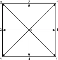
Fig.1 Discrete lattice and the particle trajectories

1.2Lattice Boltzmann model

The MRT LBE is used to solve the governing equations. In the proposed model, the space is discretized into a square lattice, with nine discrete velocities, which are given by ( see Fig.1)

Table1 The transformation matrix

The MRT lattice Boltzmann method involves two steps, i.e., a collision step and a streaming step, which can be expressed as:

Collison and forcing

The definition of the velocity is modified according to the Guo-Zheng-Shi model. Thus, the velocityandthe water depthare defined in terms of the distribution function as

Using the Chapman-Enskog procedure, Eqs.(1)-(2) can be recovered and the viscosity is

The LBSW on curvilinear coordinates is developed using the GILBM[9], based on the idea of ISLBM[5,6]. The GILBM involves three steps: the relaxation, the advection, and the interpolation. The first two steps are exactly the same as those in the previous standard LBE models. The physical and computational planes are described asrespectively. The two-step Runge-Kutta method is used to integrate the particle velocity and the second-order upwind quadratic interpolation is used for the overall interpolation process to maintain the second order approximation.

1.3Boundary conditions

In this study, we use the non-equilibrium extrapolation method[11], which is of the second order accuracy, on the inflow, outflow, and wall boundaries

The macroscopic velocities can be estimated using the neighboring fluid velocities at the slip wall and they are equal to zero at the non-slip wall.

In the turbulent flows, a large flow gradient exists in the vicinity of a solid boundary due to the wall friction, which cannot be simulated correctly with no-slip or slip boundary conditions. Thus, semi-slip boundary conditions are needed. The wall shear stressmay be represented by

2. Model accuracy

The second order accuracy of the proposed model is examined based on the Taylor-Couette flow between two circular cylinders using a curvilinear coordinate grid. The inner cylinder of radiusrotates with a constant tangential velocityand the outer cylinder of radiusis kept stationary. The radius ratioand the initial water depthThe flows with different Reynolds numbersof 10, 20 and 30 are considered.

The periodic condition is implemented on the open boundaries. Three different grid resolutions are tested with uniform meshes of 90×23, 140×36 andThe particle velocityin all cases andis the minimum grid size of each mesh. In this and the following sections, the criterion for the steady states is defined as

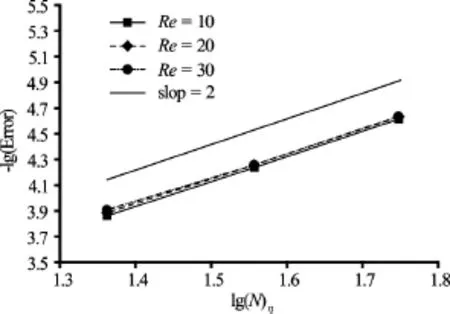
Fig.2 Errors in the velocity fields for the Taylor-Couette flow with different Reynolds numbers

With a different number of gridsin the direction, the trends in thenorm errors (calculated relative to the analytical solution[14]) for the velocity fields are quite similar in the three cases with differentnumbers (Fig.2). The asymptotical quadratic convergence is clearly seen, thereby it can be concluded that the proposed model has an overall second order accuracy in space. It should be noted that the second order boundary conditions are necessary during the simulations.

Different radius ratios are also tested, where0.2, 0.35 and 0.65 with the meshes of 140×36, 140×26 and 140×14, respectively. Figure 3 compares the simulated results and the analytical solutions, and very good agreement is observed, thereby it is concluded that the proposed curvilinear coordinate LBSW can accurately simulate the flow in a curved channel.

Fig.3 Velocity profiles of the Taylor-Couette flow for different radius ratios

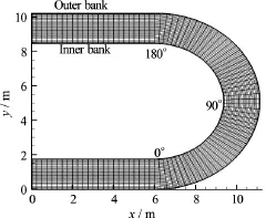
Fig.4 Computational mesh of 100×26 for thecurved channel

3. Applications

3.1Open channel flow with abend

Fig.5 Comparison of the depth-averaged velocities across the section of

Fig.6 Contours of the water depth for thecurved channel

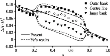
Fig.7 Water depths along the channel bend. The longitudinal distance from the inlet is normalized with the length at the centre of the bend and the water depth is normalized as

To investigate the grid convergence, we employ two uniform meshes of 50×13 and 100×26 (Fig.4) withrespectively. The particle velocitySemi-slip boundary conditions are set at the channel bank where the roughness coefficient. Figure 5 shows that with the model, similar results are obtained with different meshes where the grid convergence index(GCI, as proposed by Roache[16]) of the velocities is 1.24% for the fine mesh. These results indicate that the fine mesh can be used without large numerical errors and thus it is employed in this test.

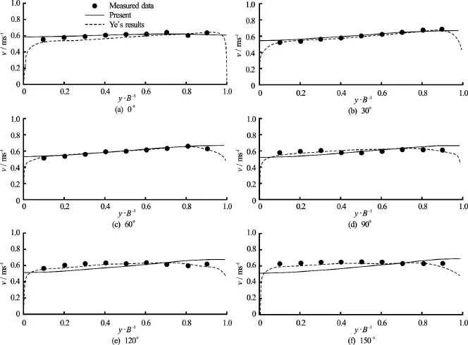
Fig.8 Depth-averaged velocity distributions on different sections

The water depth contours are illustrated in Fig.6, which are very similar to the simulated results obtained in the previous studies[17,18]. Figure 7 also compares the results obtained at the central line andof the outer bank and the inner bank. The maximum relative error at the inner bank is 2.9%. Compared with the simulated results obtained by Yeʼs 3-D FVM[19], better agreement is obtained by Yeʼs method. However, our 2-D scheme shows reasonable accuracy. In Fig.8, further comparisons between the predicted and measured depth-averaged velocities on six cross-sections show that the results obtained by the proposed model agree well with the experimental data, except for some discrepancies on the section with. In addition, the results obtained by the 3-D model are better than those obtained with the proposed 2-D model, which may have several possible explanations, as follows: (1) with the 3-D model, the secondary flow in the meandering channel can be simulated more accurately, (2) in Yeʼs study, the turbulent viscosity is more accurate because theturbulence model is employed, or (3) with a low turbulence Reynolds number, the wall region is simulated correctly by the wall function method proposed by Ye. However, our proposed model is simple and efficient, with a reasonable accuracy.

Fig.9 Computational mesh of 160×20 for two bends in themeandering channel

3.2Open channel flow withconsecutive bends

In this test, we consider the experimental channel studied by Tamai et al.[20], which involves 90° consecutive bends with a rectangular cross-section. Each bend is connected by a 0.3 m straight reach. The radius of the channel centerline is 0.6 m and the channel width. The inflow discharge is 0.002 m3/s and the constant water depth, as specifically at the outflow. The longitudinal bed slope is 1/1000 and the Manning’s roughness coefficient forthe channel is estimated to be 0.013. Thein this test.

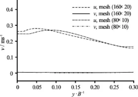
Fig.10 Comparison of the depth-averaged velocities across Section E

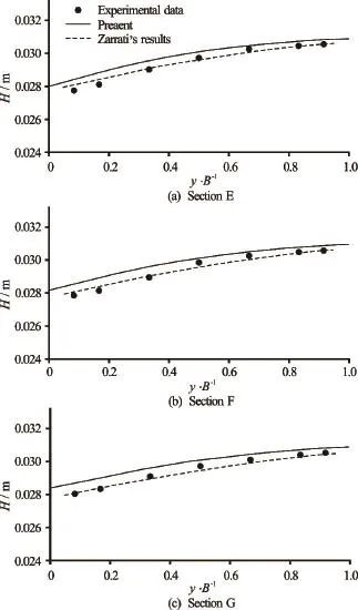
Fig.11 Water depths in the meandering channel withbends

Fig.12 Transverse profiles of the depth-averaged velocity components across three sections of the meandering channel withbends

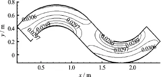
Fig.13 Contours of the water depths in the meandering channel withbends

Two meshes of 80×10 and 16×20 (see Fig.9) withrespectively, are tested. The results obtained by using the two different mesh resolutions are shown in Fig.10.Compared with the coarse mesh (80×10), the GCI for the fine mesh (160×20) is only 0.3% in terms of the depth-averaged velocities, so the fine mesh can be used.

Fig.14 Contours of the water depth in the meandering channel withbends

Fig.15 Water depths in the meandering channel withbends

The water depths and the depth-averaged velocity profiles on Sections E, F and G are plotted in Figs.11, 12, respectively. Good agreement is observed for the water depth, where the maximum relative error is 2.8%. There are some differences in the velocity distribution, but the numerical results for the longitudinal and lateral velocities agree well with the experimental data. Compared with the simulations reported by Zarrati et al.[21], obtained by using a 2-D depth-averaged FVM model with a nonorthogonal curvilinear coordinate system, it is found that our method gives very similar results (the maximum relative error in the water depth is 1.5% according to Zarrati et al). The overall agreement is good between the results obtained by using our proposed method and the solutions reported by Zarrati et al.. After reaching a steady state, the water depth increases from the inner bank to the outer bank and it becomes almost constant at the straight reach (see Fig.13), as in good agreement with the experimental results.

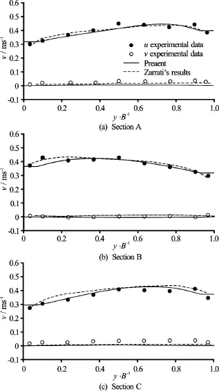
Fig.16 Transverse profiles of the depth-averaged velocity components across three sections of the meandering channel withbends

3.3Open channel flow withconsecutive bends

In the final test, we consider awide meandering rectangular channel with an angle ofThere are 18 circular bends and each bend is connected by a 0.07 m straight reach. The radius of the channel centerline is 1.3 m. The discharge rate isand the average flow depth0.045 m. The Manning’s roughness coefficient and the longitudinal gradient of the channel are 0.008 and 1/1 000, respectively.

A uniform 192×15 mesh is used to calculate four consecutive bends, whereThe roughness coefficientin the semi-slip boundary conditions is 1.1032.

The water depth contours are plotted in Fig.14, and it is shown that the water depth increases from the inner bank to the outer bank due to the centripetal force. Figures 15, 16 show the water depths and the depth-averaged velocity profiles on Sections A, B and C along the reach where we take measurements, as shown in Fig.14. An excellent agreement is observed in terms of the water depth with the relative error less than 3.0%. The predicted velocities on these three sections also agree well with the experimental results. In general, good agreement is observed between the results obtained by using the proposed method and the solutions reported by Zarrati et al. (the maximum relative error of water depth is 2.0% according to Zarrati et al.), as shown in Figs.15, 16.

4. Conclusions

In this study, a second order LBSW is developed on a curvilinear coordinate grid, and the GILBM and MRT models are implemented. A non-equilibrium extrapolation method is used to handle the inflow, outflow and wall boundaries. It is demonstrated that the proposed model enjoys a second order accuracy in space. In general, the treatment of the wall boundaries is easier and more exact results are obtained for the meandering flows after applying the curvilinear coordinate grid. The proposed model is verified by considering the Taylor-Couette flow, where three meandering channel flows withconsecutive bends are tested. The results show that with the proposed model, reasonable depth-averaged hydrodynamic characteristics can be obtained for the shallow water flow in curved and meandering open channels over a wide range of bend angles.

第七个月，‘皮肤上长满毛毛，皮下脂肪少，皮肤皱褶，如果此时出生，能啼哭与吞咽，但生活力弱。’”[11]

The proposed model can be used to solve more complex practical problems such as for curved and meandering rivers. The turbulent models and other boundary treatments such as the wall function method, can also be integrated to solve more complex flow problems. Moreover, the advection and anisotropic dispersion equations can be coupled to solve the advection-dispersion problems. These extensions and further applications will be considered in our future research.

[1] Zhao Z., Huang P., Li Y. et al. A lattice Boltzmann method for viscous free surface waves in two dimensions [J].International Journal for Numerical Methods in Fluids, 2013, 71(2): 223-248.

[2] Zhao Z. M., Huang P., Chen L. P. Lattice Boltzmann method for simulating viscous free surface waves in three dimensions [J].ChineseJournal of Hydrodynamics, 2013, 28(6): 708-716(in Chinese).

[3] Li S., Huang P., Li J. A modified lattice Boltzmann model for shallow water flows over complex topography [J].International Journal for Numerical Methods in Fluids, 2014, 77(8): 441-458.

[4] Zhang C. Z., Cheng Y. G., Wu J. Y. et al. Lattice Boltzmann simulation of the open channel flow connecting two cascaded hydropower stations [J].Journal of Hydrodynamics, 2016, 28(3): 400-410.

[5] He X., Luo L., Dembo M. Some progress in lattice Boltzmann method. Part I. Nonuniform mesh grids [J].Journal of Computational Physics, 1996, 129(2): 357-363.

[6] He X., Luo L., Dembo M. Some progress in the lattice Boltzmann method: Reynolds number enhancement in simulations [J].Physical A, 1997, 239(1-3): 276-285.

[7] Budinski L. MRT lattice Boltzmann method for 2D flows in curvilinear coordinates [J].Computers and Fluids, 2014, 96: 288-301.

[8] He X., Doolen G. Lattice Boltzmann method on curvilinear coordinates system: Flow around a circular cylinder [J].Journal of Computational Physics, 1997, 134(2): 306-315.

[9] Imamura T., Suzuki K., Nakamura T. et al. Acceleration of steady-state lattice Boltzmann simulations on non-uniform mesh using local time step method [J].Journal of Computational Physics, 2005, 202(2): 645-663.

[10] Tubbs K. Lattice Boltzmann modeling for shallow water equations using high performance computing [C]. Doctoral Thesis, Baton Rouge, USA: Louisiana State University, 2010.

[11] Guo Z. L., Zheng C. G., Shi B. C. Non-equilibrium extrapolation method for velocity and pressure boundary conditions in the lattice Boltzmann method [J].Chinese Physics, 2002, 11(4): 366-374.

[12] Guo Z., Zheng C. Analysis of lattice Boltzmann equation for microscale gas flows: Relaxation times, boundary conditions and the Knudsen layer [J].International Journal of Computational Fluid Dynamics, 2008, 22(7): 465-473.

[13] Du R., Shi B., Chen X. Multi-relaxation-time lattice Boltzmann model for incompressible flow [J].Physics Letters A, 2006, 359(6): 564-572.

[14] Chen M. Fundamentals of viscous fluid dynamics [M]. Beijing, China: China Higher Education Press, 2002(in Chinese).

[15] Vriend H. D. A mathematical model of steady flow in curved shallow channels [J].Journal of Hydraulic Research, 1977, 15(1): 37-54.

[16] Roache P. Perspective: A method for uniform reporting of grid refinement studies [J].Journal of Fluids Engineering, 1994, 116(3): 405-413.

[17] Duan J. G. Simulation of flow and mass dispersion in meandering channels [J].Journal of Hydraulic Engineering, ASCE, 2004, 130(10): 964-976.

[18] Zhang M. L., Shen Y. M. Three-dimensional simulation of meandering river based on 3-D RNGturbulence model [J].Journal of Hydrodynamics, 2008, 20(4): 448-455.

[19] Ye J., Mccorquodale J., Barron R. A three-dimensional hydrodynamic model in curvilinear co-ordinates with collocated [J].International Journal for Numerical Methods in Fluids, 1998, 28(7): 1109-1134.

[20] Tamai N., Ikeuchi K., Yamazaki A. et al. Experimental analysis on the open channel flow in rectangular continuous bends [J].Journal of Hydroscience and Hydraulic Engineering, 1983, 1(2): 17-31.

[21] Zarrati A., Tamai N., Jin Y. Mathematical modeling of meandering channels with a generalized depth averaged model [J].Journal of Hydraulic Engineering, ASCE, 2005, 131(6): 467-475.

[22] Tarekul Islam G., Tamai N., Kobayashi K. Hydraulic characteristics of a doubly meandering compound channel [C].Proceedings of Joint Conference on Water Resource Engineering and Water Resources Planning and Management 2000. Minneapolis, USA: ASCE, 2000, 1-9.

(Received January 12, 2015, Revised August 30, 2015)

* Project supported by the Chinese Special Fund for Environmental Protection Research in the Public Interest (Grant No. 201309006).

Biography: Zhuang-ming Zhao (1986-), Male, Ph. D.