Tae Uk Jang, Yue-bin Wu (伍悦滨), Ying Xu (徐莹), Qiang Sun (孙强)

1.Department of Mechanics, Kim Il Sung University, Pyong Yang, D. P. R. Korea

2.School of Municipal and Environmental Engineering, Harbin Institute of Technology, Harbin 150090, China,

E-mail: jtu_rns @163.com

3.State Key Laboratory of Urban Water Resource and Environment, Harbin Institute of Technology, Harbin 150090, China

4.School of Energy and Architecture, Harbin University of Commerce, Harbin 150028, China

A scheme for improving computational efficiency of quasi-two-dimensional model＊

Tae Uk Jang1,2, Yue-bin Wu (伍悦滨)2,3, Ying Xu (徐莹)4, Qiang Sun (孙强)2

1.Department of Mechanics, Kim Il Sung University, Pyong Yang, D. P. R. Korea

2.School of Municipal and Environmental Engineering, Harbin Institute of Technology, Harbin 150090, China,

E-mail: jtu_rns @163.com

3.State Key Laboratory of Urban Water Resource and Environment, Harbin Institute of Technology, Harbin 150090, China

4.School of Energy and Architecture, Harbin University of Commerce, Harbin 150028, China

The quasi-2D model, taking into account the axial velocity profile in the cross section and neglecting the convective term in the 2-D equation, can more accurately simulate the water hammer than the 1-D model using the cross-sectional mean velocity. However, as compared with the 1-D model, the quasi-2D model bears a higher computational burden. In order to improve the computational efficiency, the 1-D method is proposed to be used to solve directly the pressure head and the discharge in the quasi-2D model in this paper, based on the fact that the pressure head obtained as the solution of the two-dimensional characteristic equation is identical to that solved by the 1-D characteristic equations. The proposed scheme solves directly the 1-D characteristic equations for the pressure head and the discharge using the MOC and solves the 2-D characteristic equation for the axial velocities in order to calculate the wall shear stress. If the radial velocity is needed, it can be evaluated easily by an explicit equation derived from the explicit 2-D characteristic equation. In the numerical test, the accuracy and the efficiency of the proposed scheme are compared with two existing quasi-two-dimensional models using the MOC. It is shown that the proposed scheme has the same accuracy as the two quasi-2D models, but requires less computational time. Therefore, it is efficient to use the proposed scheme to simulate the 2-D water hammer flows.

Water hammer, method of characteristics, numerical scheme, pipe, quasi-2D model

Introduction

The water hammer is a widespread phenomenon in water supply pipeline systems, which often poses a threat to the safety of the pipeline systems, so it is important to simulate the water hammer at the design stage as well as during the operation of the water supply networks[1-3]. Due to easy programming and high computational efficiency, the 1-D model is widely used for the analysis of water hammer problems[4]. However, the 1-D model underestimates the frictional resistances by using a steady or quasi-steady friction term[5-7]. In fact, the velocity gradients at the wall of the pipe are greater in the unsteady flows and thus, the wall shear stresses are larger than the corresponding values in the steady flows[8]. In order to simulate the water hammer flows accurately, a 2-D model or a quasi-2D model should be used. The quasi-2D model[9,10], based on the assumption that the flow is axially symmetric and the convective terms are negligible, associates the 1-D pressure distribution with the 2-D velocity distribution. Because the velocity profiles are taken account of in the cross section, the quasi-2D model simulates the water hammer more accurately than the 1-D model. However, it bears a higher com-putational burden. Therefore, it is necessary to improve the computational efficiency of the quasi-2D model.

Several numerical schemes were applied to quasi-2D models for analysis of water hammer problems. Vardy and Hwang[11]solved the hyperbolic part of 2-D governing equations by the method of characteristics (MOC) and the parabolic part by finite difference (FD). The model of Vardy and Hwang is known to be accurate and stable[12,13], however, it involves the inversion of a large matrix. Silva-Araya and Chaudhry[14]proposed a scheme to solve the governing equations in the 1-D framework by MOC and the 2-D momentum equation by FD. Pezzinga[5,15]used the explicit FD scheme to solve the 1-D continuity equation and the implicit FD scheme to solve the 2-D momentum equation. The model is efficient due to the decoupling between the 1-D continuity and 2-D momentum equations, through ignoring the radial velocity in the calculation process and evaluating the discharge by numerical integration. Zhao and Ghidaoui[16]proposed an efficient quasi-2D model to improve the numerical efficiency in the model of Vardy and Hwang, which requires the calculation of two smaller tri-diagonal matrices. The model of Zhao and Ghidaoui, with the consideration of the effect of the radial velocity component, is a stable implicit scheme. Wahba[17]proposed a scheme to solve the 1-D continuity equation and the 2-D momentum equation by FD for analysis of water hammer flows in the low Reynolds number range. Korbar et al.[18,19]proposed an efficient scheme to improve the numerical efficiency of the Zhao and Ghidaoui model. In this model, the axial velocity was evaluated using the 2-D characteristic equation and the pressure head was calculated using the 1-D characteristic equation.

This paper proposes to solve directly the pressure head and the discharge in the 1-D form and the wall shear stress in the 2-D form by MOC, based on the fact that the pressure head obtained by the 2-D characteristic equation is identical to that by the 1-D characteristic equations. The accuracy and the efficiency of the proposed scheme are shown by comparing with the two quasi-2D models (i.e., the model of Zhao and Ghidaoui and the model of Korbar et al.) in a numerical test.

1. Governing equations and numerical scheme

1.1Governing equations of quasi-2D model

Assuming that the flow is axially symmetric and the convective terms are negligible, the 2-D governing equations for water hammer flows in a pipe are expressed as follows[16]:

1.2Quasi-2D models

The computational domain for the discretization of Eq.(5) is shown in Fig.1. The pipe length,, is divided intoreaches with a constant lengthin the axial direction. Each computational point in the axial direction of the pipe is discretized intocylinders with varying thickness in the radial direction. In Fig.1(a),are the coordinates of theboundary and middle points of reaches in the radial direction, respectively. The axial velocity,u, is located at the middle of each radial reach, whereas the radial velocityand the turbulent viscosityare located at the boundaries of each radial reach. The time stepThe subscriptsandare the indexes of grid points in the axial and radial directions, respectively. The superscriptindicates the time level.

Fig.1 Radial and MOC grid systems

Integrating Eq.(5) over the characteristic lines betweenthe discretized forms of Eq.(5) become

where the weight coefficientsare for the temporal discretization of the viscous and radial velocity terms in Eq.(5), respectively. Using the central difference scheme for both the viscous and radial flux terms in the above equations, the resulting equations are expressed as[16]

1.3Proposed numerical scheme

In the proposed scheme, the axial velocities are evaluated by Eq.(11) as the quasi-2D model of Zhao and Ghidaoui, but both the pressure head and the radial flux are obtained from the explicit equations instead of using Eq.(12). In fact, it is proved mathematically that the pressure head obtained as the solution of Eq.(12) is identical to that obtained by using the 1-D characteristic equation. Eq.(12) for the pressure head and the radial flux may be rewritten as

Therefore, the pressure head from Eq.(17) may be written as

Using the expression of the coefficient, the denominator term on the right side of Eq.(18) may be expressed as

If the number of radial reaches is sufficiently large, the cross-sectional area of the pipe,and the discharge,calculated by numerical integration are given by

Therefore, Eq.(22) leads to the following equation

Equation (22) is identical to the equation for the pressure head obtained by using the 1-D characteristic equation (i.e., Eq.(6)). Therefore, the pressure head in the proposed scheme is solved by the 1-D characteristic equation. The discharge is also solved by the 1-D characteristic equation and may be expressed as

The wall shear stress at each point at each time may be evaluated by the following equation

Once the pressure head is determined, if needed, the radial flux may be easily calculated by using Eq.(13).

Therefore, it is shown that, for the quasi-2D model, the pressure and the discharge can be solved by the 1-D equation and the shear stress is obtained by the 2-D equation. In this paper, the 1-D and 2-D governing equations are solved by using MOC in the scheme.

2. Numerical test

The proposed scheme and the two quasi-2D models (i.e., the Model (I) refers to the model of Zhao and Ghidaoui and the Model (II) refers to the model of Korbar et al.) are applied to a numerical test. The water hammer is caused by an instantaneous downstream valve closure in a reservoir-pipe-valve system. The following geometric and flow parameters are used for the numerical test: the length of the pipe,is 900 m, the diameter of the pipe,is 0.5 m, the wave speed,is 900 m/s, the steady discharge,, is 0.5 m3/s, the steady head of the reservoir,, is 67.7 m, the kinetic viscosity,and the Reynolds number,

2.1Comparison of accuracies

The accuracy of the proposed scheme is evaluated by comparing the results with the Models (I) and (II). Figure 2 shows the pressure head traces at the midpoint of the pipe calculated by the proposed scheme, the Model (I) and the Model (II), using the weight coefficientson the gridAs is expected, the results obtained by the proposed scheme are almost the same as those of the two models.

Fig.2 Pressure head traces at mid-point of pipe calculated by proposed scheme and two models

Fig.3 Maximal error between both pressure heads calculated by proposed scheme and Model (I)

Figure 3 shows the maximal errors between the pressure heads calculated by the proposed scheme and the Model (I), using the weight coefficientson different grids. The maximal error between both pressure heads is evaluated by the following equation

Figure 4 shows the discharge changes at the upstream reservoir calculated by the proposed scheme and the Model (II). As is expected, the discharge obtained by the proposed scheme is almost identical to that calculated by the Model (II).

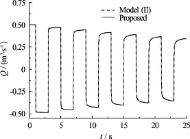
Fig.4 Discharge traces at upstream reservoir calculated by proposed scheme and Model (II)

Fig.5 Maximal error between both discharges calculated by proposed scheme and Model (II)

Figure 5 shows the maximal errors between discharges calculated by both the present scheme and the Model (II), using the weight coefficientson different grids. The maximal error between both discharges is calculated by the following equation

Figure 6 shows the wall shear stress traces at the mid-point of the pipe obtained by the proposed scheme and two models. Obviously, the wall shear stress calculated by the present scheme is almost identical to that of the two models.

Fig.6 Wall shear stress traces at mid-point of pipe calculated by proposed scheme and two models

Fig.7 Maximal error between both wall shear stresses calculated by proposed scheme and Model (I)

Figure 7 shows the maximal errors between the wall shear stresses calculated by both the present scheme and the Model (I), using the weight coefficientson different grids. The maximal error between both wall shear stresses is evaluated by

Figure 8 shows the velocity profiles at the midpoint of the pipe at the specified time calculated by the proposed scheme and the two models. Obviously, the velocity profiles obtained by the proposed schemeare almost identical to those obtained by the Models (I) and (II).

Fig.8 Velocity profiles at mid-point of pipe calculated by proposed scheme and two models

Fig.9 CPU time ratio between the proposed scheme to the Model (I) on different grids

Fig.10 CPU time ratios between the proposed scheme to the Model (II) on different grids

2.2Comparison of computational efficiencies

The computational efficiency of the proposed scheme is compared with the Models (I) and (II), using the same weight coefficients on the same grid. Figure 9 shows the CPU time ratio of the proposed scheme to the Model (I) on the different grids. For two different weight coefficients, the results show that, regardless of the grid size, the proposed scheme takes less computational time than the Model (I). In all cases, the required CPU time for the proposed scheme is approximately 93% of that for the Model (I). Figure10 shows the CPU time ratio between the proposed scheme to the Model (II). In Fig.10, the proposed scheme generally takes less computational time than the Model (II) using the same weight coefficients. In all cases, the proposed scheme takes about 66% of the CPU time required for the Model (II).

The present scheme generally takes less computational time than the Models (I) and (II), regardless of the grid size. Because in the proposed scheme, explicit equations are used to calculate the pressure head and the radial flux, the computational time is reduced with respect to the matrix calculation in the Model (I). In addition, the use of explicit equations for the discharge also reduces the computational time with respect to the discharge calculation by numerical integration of the axial velocity profile in the Model (II). However, the velocity profiles are still calculated by a tri-diagonal matrix (i.e., Eq.(11)) and thus, the proposed scheme still takes longer computational time than the 1-D model. If the velocity profiles are obtained by a simpler way, the proposed scheme will be more efficient for simulating 2-D water hammer flows.

3. Conclusion

This paper proposes to use the 1-D method to directly solve the pressure head and the discharge in the quasi-2D model, based on the fact that the pressure head obtained by solving the 2-D characteristic equation is identical to that obtained by solving 1-D characteristic equation. The proposed scheme is used to solve directly the 1-D characteristic equation for the pressure head and the discharge using the MOC, while the 2-D characteristic equation is only used for the axial velocities in order to calculate the wall shear stress. If the radial velocity is needed, it can be evaluated easily by an explicit equation derived from the 2-D characteristic equation. The numerical test shows that, for the same weighting coefficients and grids, the proposed scheme gives the same results as the quasi-2D models in the numerical tests. The present scheme generally requires less computational time than the quasi-2D models, regardless of the grid size. In all cases, the proposed scheme takes about 93% and 66% of the required CPU times for the model of Zhao and Ghidaoui and the model of Korbar et al., respectively. Therefore, the proposed scheme is an efficient scheme for analyzing the 2-D water hammer flows.

[1] Yu K., Cheng Y. G., Zhang X. X. Hydraulic characteristics of a siphon-shaped overflow tower in a long water conveyance system: CFD simulation and analysis [J].Journal of Hydrodynamics, 2016, 28(4): 564-575.

[2] Sun Q., Wu Y. B., Xu Y. et al. Optimal sizing of an air vessel in a long-distance water-supply pumping system using the SQP method [J].Journal of Pipeline Systems Engineering and Practice, 2016, 7(3): 05016001.

[3] Sun Q., Wu Y. B., Xu Y. et al. Flux vector splitting schemes for water hammer flows in pumping supply systems with air vessels [J].Journal of Harbin Institute of Technology (New Series), 2015, 22(3): 69-74.

[4] Chaudhry M. H. Applied hydraulic transients [M]. 3rd Edition, New York, USA: Van Nostrand Reinhold, 2014.

[5] Pezzinga G. Evaluation of unsteady flow resistances by quasi-2D or 1D models [J].Journal of Hydraulic Engineering, ASCE, 2000, 126(10): 778-785.

[6] Shimada M., Vardy A. E. Nonlinear interaction of friction and interpolation errors in unsteady flow analyses [J].Journal of Hydraulic Engineering, ASCE, 2013, 139(4): 397-409.

[7] Vitkovsky J. P., Bergant A., Simpson A. R. et al. Systematic evaluation of one-dimensional unsteady friction models in simple pipelines [J].Journal of Hydraulic Engineering, ASCE, 2006, 132(7): 696-708.

[8] Vardy A. E., Brown J. M. B. Approximation of turbulent wall shear stresses in highly transient pipe flows [J].Journal of Hydraulic Engineering, ASCE, 2007, 133(11): 1219-1228.

[9] Jang T. U., Wu Y. B., Xu Y. et al. Efficient quasi-twodimensional water hammer model on a characteristic grid [J].Journal of Hydraulic Engineering, ASCE, 2016, 142(12): 06016019.

[10] Tazraei P., Riasi A. Quasi-two-dimensional numerical analysis of fast transient flows considering non-Newtonian effects [J].Journal of Fluids Engineering, 2016, 138(1): 011203.

[11] Vardy A. E., Hwang K. L. A characteristics model of transient friction in pipes [J].Journal of Hydraulic Research, 1991, 29(5): 669-684.

[12] Jang T. U., Wu Y. B., Xu Y. et al. Numerical simulation for two-phase water hammer flows in pipe by quasi-twodimensional model [J].Journal of Harbin Institute of Technology (New Series), 2016, 23(2): 9-15.

[13] Zhao M. Numerical solutions of quasi-two-dimensional models for laminar water hammer problems [J].Journal of Hydraulic Research, 2016, 54(3): 360-368.

[14] Silva-Araya W. E., Chaudhry M. H. Computation of energy dissipation in transient flow [J].Journal of Hydraulic Engineering, ASCE, 1997, 123(2): 108-115.

[15] Pezzinga G., Brunone B., Meniconi S. Relevance of pipe period on kelvin-voigt viscoelastic parameters: 1D and 2D inverse transient analysis [J].Journal of Hydraulic Engineering,ASCE, 2016, 142(12): 04016063.

[16] Zhao M., Ghidaoui M. S. Efficient quasi-two-dimensional model for water hammer problems [J].Journal of Hydraulic Engineering, ASCE, 2003, 129(12): 1007-1013.

[17] Wahba E. M. Turbulence modeling for two-dimensional water hammer simulations in the low Reynolds number range [J].Computers and Fluids, 2009, 38(9): 1763-1770.

[18] Korbar R., Virag Z., Savar M. Efficient solution method for quasi two-dimensional model of water hammer [J].Journal of Hydraulic Research, 2014, 52(4): 575-579.

[19] Korbar R., Virag Z., Savar M. Truncated method of characteristics for quasi-two-dimensional water hammer model [J].Journal of Hydraulic Engineering, ASCE, 2014, 140(6): 04014013.

(Received January 7, 2015, Revised November 2, 2015)

* Project supported by the National Natural Science Fund in China (Grant No. 51208160), the Foundation for Distinguished Young Talents in Higher Education of Heilongjiang Province (Grant No. UNPYSCT-2015072) and the Harbin Science and Technology Project.

Biography: Tae Uk Jang (1962-), Male, Ph. D.,

Associate Professor

Yue-bin Wu,

E-mail: ybwu@hit.edu.cn